𝗕𝗶𝘁𝗰𝗼𝗶𝗻 𝗣𝗿𝗶𝗰𝗲 𝗣𝗿𝗲𝗱𝗶𝗰𝘁𝗶𝗼𝗻 𝘄𝗶𝘁𝗵 𝗟𝗦𝗧𝗠

(Long Short Term Memory networks)

Video in my YouTube Channel explaining step by step the whole project of building an LSTM prediction model from BTC-USD historical price data from 2015–2021.

Link to full NoteBook in my Kaggle

Full Code at Github

Basic Architecture of LSTM

LSTMs are a type of recurrent neural network, but instead of simply feeding its outcome into the next part of the network, an LSTM does a bunch of math operations so it can have a better memory.

A typical LSTM network is comprised of different memory blocks called cells (the rectangles that we see in the image). There are two states that are being transferred to the next cell; the cell state and the hidden state. The memory blocks are responsible for remembering things and manipulations to this memory is done through three major mechanisms, called gates.

• Unlike standard feedforward neural networks, LSTM has feedback connections. It can process not only single data points, but also entire sequences of data.

• LSTMs are explicitly designed to avoid the long-term dependency problem. Remembering information for long periods of time is practically their default behavior, not something they struggle to learn like RNNs!

• Also, they don’t suffer from problems like vanishing/exploding gradient descent.

When should I use an RNN LSTM and when to use ARIMA for a time series forecasting problem

If the data follow linear relationships ARIMA gives acceptable results.

And if data also has non-linear relationships RNN (depending on the activation function) tend to give better results.

In theory RNN should also be able to model linear relationships in the data, however the ARIMA model is “simple” compared to the RNN.

After applying the ARIMA model to your data, you can test for non modeled non-linear relationships in the residuals with the Lee, White and Granger (LWG) test. If there are non-linear relationships in the residuals maybe you should use a more capable non-linear model like RNN.

Now a slightly more granular analysis on when to use RNN / LSTM vs simple ARIMA

There is one thing about deep models that promises better productivity by eliminating the data scientist/statistician. Its like you can throw the kitchen sink (all data in your ERP) in, and it will do the feature discovery for you. This is somewhat reasonable because that’s what happened for high-frequency signals (image, audio, sound). However, typical time series are not signals in the sense of being samples of levels of some physical quantity that can be sampled arbitrarily densely. They are aggregates.

In time series, you have uncertainty about future values. So the question that needs to be asked, in this series of data, is the uncertainty stochastic or epistemic kind?

If the series has truly random behavior, use a probabilistic model. ARIMA-type models have implicit Gaussian assumptions and are a good maximum entropy default.

If the series is highly determined but the generating process is inscrutably complex, it will look random. Here, use a model that has a better chance of picking that process up. Something like an RNN.

There is usually some mix of stochastic (truly random) and epistemic (don’t know everything there is to know about the generating process) variation. There isn’t much you can do about the stochastic component, so focus on getting better information about the process.

Video in my YouTube Channel to explain the whole project of building an LSTM model from BTC-USD historical data from 2015–2021

Link to full NoteBook in my Kaggle

Full Code at Github

---

Further ways to improve Model Accuracy by adding extra features

For this, there are quite a few options.

1. First of all, in the video above, for the sake of simplicity, I only created a single dimensional model using the Close price only.

I could use all of Open, High, Low, Close and Volume to predict the Closing prices. And that would be a MULTIDIMENSIONAL LSTM prediction, which could have improved the accuracy of the model.

2. Further ideas to include features / input variables to the model, might be to include technical indicators on Bitcoin prices.

Examples, Simple Moving Average (SMA), Moving Average Convergence-Divergence Indicator (MACD), Stochastic Oscillator, Relative Strength Index (RSI), Average Directional Index (ADX), On-Balance-Volume (OBV), Average Directional Index (ADX). These are some of the top ones. I am including a basic Python code for SMA and RSI below

4. Then according to this Study (link below) they have got best results by utilizing as inputs different cryptocurrency data ( BTC, ETH and Ripple (XRP)) and handles them independently in order to exploit useful information from each cryptocurrency separately. So basically historical prices of other related cryptos are also an input to the model for the Crypto that you are tyring to predict.

Study Link - => https://d-nb.info/1185667245/34

---

Python code for SMA and RSI below

Simple Moving Average (SMA)

The Simple Moving Average (SMA) is calculated by adding the price of an instrument over a number of time periods and then dividing the sum by the number of time periods. The SMA is basically the average price of the given time period, with equal weighting given to the price of each period.

Formula

SMA = ( Sum ( Price, n ) ) / n

Where: n = Time Period

def simple_moving_average(df, periods=25):
    """
    Simple Moving Average for the past n days.
    Values must be descending
    """
    last_n_days_sma = []

    for i in range(len(df)):
        if i < periods:

            # Appending NaNs for instances unable to look back on
            last_n_days_sma.append(np.nan)

        else:
            # Otherwise calculate the SMA
            last_n_days_sma.append(round(np.mean(df[i:periods+i]), 2))

    return last_n_days_sma

RSI

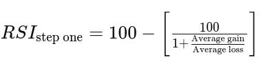
def relative_strength_index(df, periods=14):
    """
    Relative Strength Index
    **Values must be descending**
    """

    df = df.diff()

    last_n_days_rsi = []

    for i in range(len(df)):
        if i < periods:

            # Appending NaNs for instances unable to look back on
            last_n_days_rsi.append(np.nan)

        else:

            # Calculating the Relative Strength Index
            avg_gain = (sum([x for x in df[i:periods+i] if x >= 0]) / periods)
            avg_loss = (sum([abs(x) for x in df[i:periods+i] if x <= 0]) / periods)


            rs = avg_gain / avg_loss

            rsi = 100 - (100 / (1 + rs))

            last_n_days_rsi.append(round(rsi, 2))


    return last_n_days_rsi