All the basic Matrix Algebra you will need in Data Science
The must know Matrix concepts you need as a Machine Learning Engineer

Matrix Basic Definitions
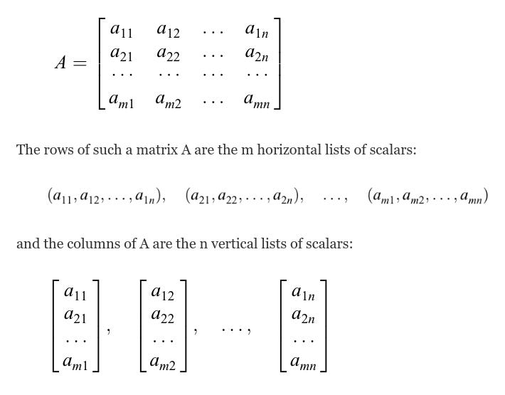
A matrix A over a field K or, simply, a matrix A (when K is implicit) is a rectangular array of scalars usually presented in the following form:
A matrix with m rows and n columns is called an m by n matrix, written as mn. The pair of numbers m and n is called the size of the matrix. Two matrices A and B are equal, written A = B, if they have the same size and if corresponding elements are equal. Thus, the equality of two m* n matrices is equivalent to a system of m* n equalities, one for each corresponding pair of elements.

Matrix vs Vectors
A matrix is simply a rectangular array of numbers and a vector is a row (or column) of a matrix.
vector is one dimension array such a=[1 2 3 4 5], but the matrix is more than one dimension array, and has some of operations.
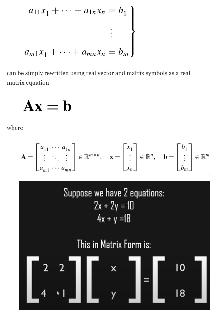
A real system of linear equations
The rank of a matrix
Matrix Multiplication
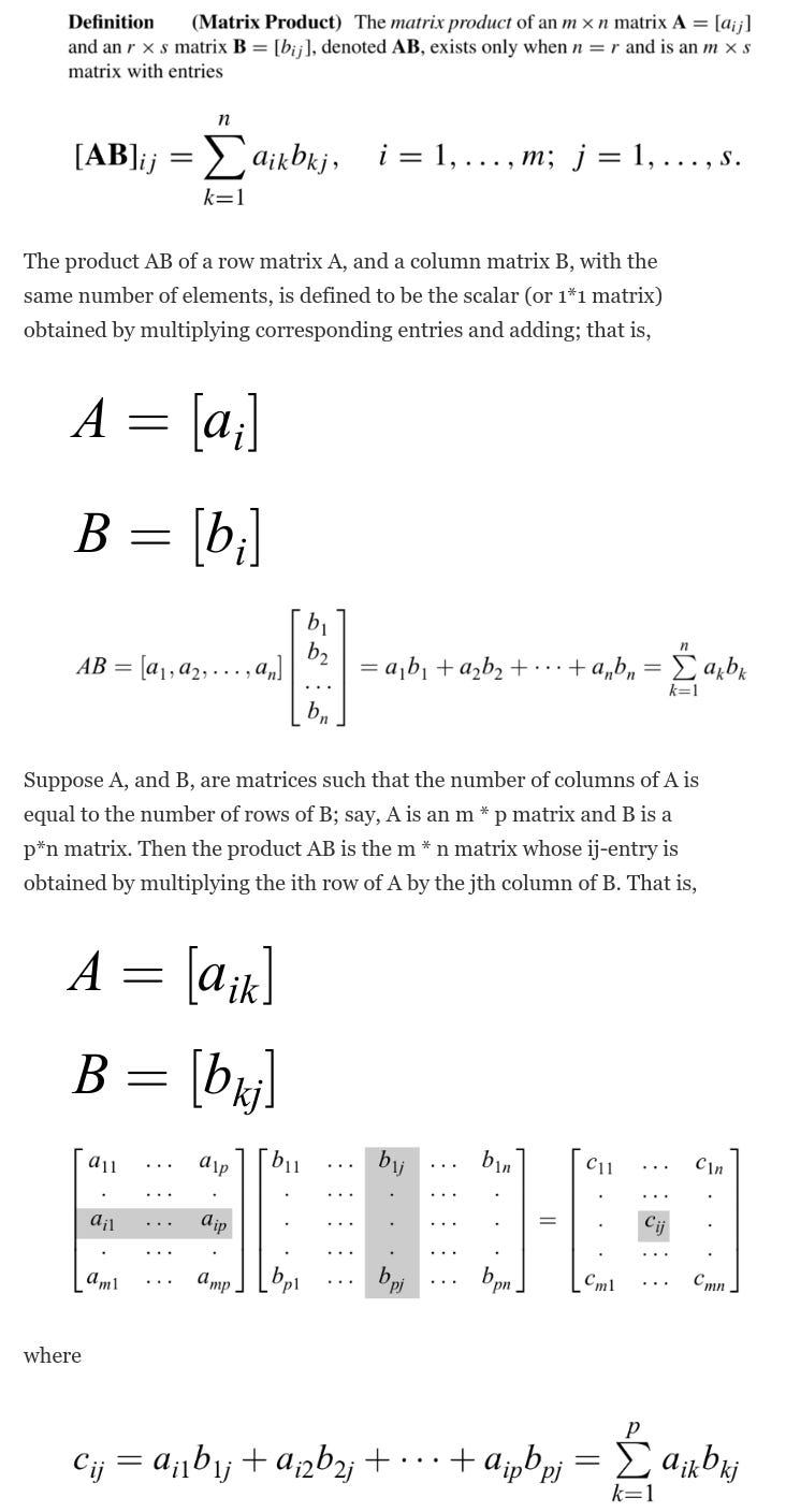
There are four simple rules that will help us in multiplying matrices, listed here:
Firstly, we can only multiply two matrices when the number of columns in matrix A is equal to the number of rows in matrix B.
Secondly, the first row of matrix A multiplied by the first column of matrix B gives us the first element in the matrix AB, and so on.
Thirdly, when multiplying, order matters — specifically, AB ≠ BA.
Lastly, the element at row i, column j is the product of the ith row of matrix A and the jth column of matrix B.
Further read through this for a very nice visual flow of Matrix Multiplication.
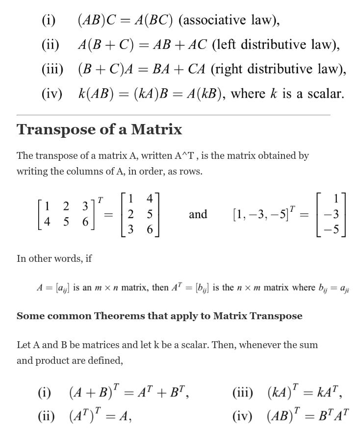
Let A; B; C be matrices. Then, whenever the products and sums are defined,
Square Matrices
A square matrix is a matrix with the same number of rows as columns. An n n square matrix is said to be of order n and is sometimes called an n-square matrix. Recall that not every two matrices can be added or multiplied. However, if we only consider square matrices of some given order n, then this inconvenience disappears. Specifically, the operations of addition, multiplication, scalar multiplication, and transpose can be performed on any nn matrices, and the result is again an n — n matrix.
The following are square matrices of order 3
Eigenvalues and Eigenvectors
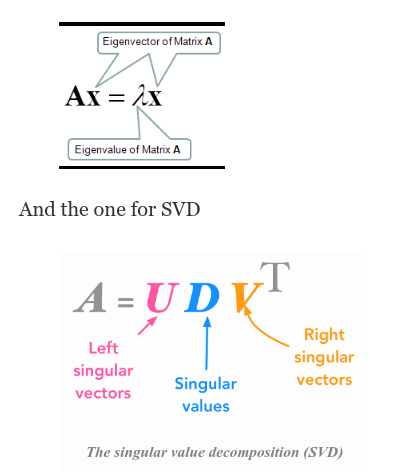
For an n × n matrix A, if the linear algebraic equation
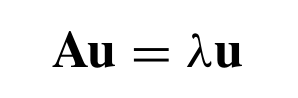
has a nonzero n × 1 solution vector u, then the scalar λ is called an eigenvalue of the matrix A, and u is its eigenvector corresponding to λ
Eigenvalues and eigenvectors are only for square matrices. Non-square matrices do not have eigenvalues. If the matrix A is a real matrix, the eigenvalues will either be all real, or else there will be complex conjugate pairs.
Eigenvectors are by definition nonzero. Eigenvalues may be equal to zero.
We do not consider the zero vector to be an eigenvector: since A0=0=λ0 for every scalar λ, the associated eigenvalue would be .
If someone hands you a matrix A and a vector v, it is easy to check if v is an eigenvector of A: simply multiply v by A and see if Av is a scalar multiple of v. On the other hand, given just the matrix A it is not so straightforward to find the eigenvectors. There are few steps involved here.
MATRIX FACTORIZATION
First note, most of the times “matrix factorization” and “matrix decomposition” are used interchangeably
Suppose we want to express an m * n matrix A as the product of two matrices A1 and A2 in the form
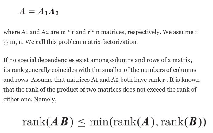
for any matrices A and B for which their product can be defined.
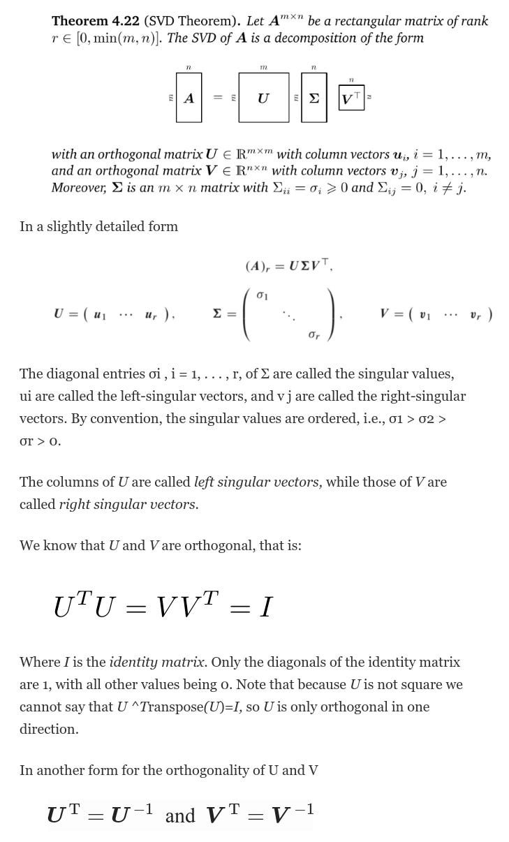
Singular Value Decomposition
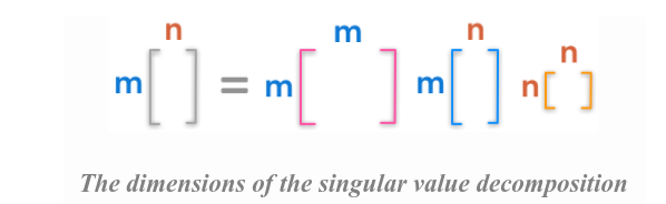
Singular value decomposition is a method of decomposing a matrix into three other matrices and its a central matrix decomposition method in linear algebra. It has been referred to as the “fundamental theorem of linear algebra”.
The SVD is used widely both in the calculation of other matrix operations, such as matrix inverse, but also as a data reduction method in machine learning. SVD can also be used in least squares linear regression, image compression, and denoising data.
Here are the dimensions of the factorization:
Interpretation of SVD
The intuition behind the singular value decomposition needs some explanations about the idea of matrix transformation.
A is a matrix that can be seen as a linear transformation. This transformation can be decomposed in three sub-transformations: 1. rotation, 2. re-scaling, 3. rotation. These three steps correspond to the three matrices U, Σ, and V.
Comparing SVD with Eigenvalues and Eigen Vectors
First noting the formulae of Eigenvalues
The key point to note here, that the concept of Singular-Value is a lot like eigenvalues, but different because the matrix A now is more usually rectangular. But for a rectangular matrix, the whole idea of eigenvalues is not possible because if I multiply A times a vector x in n dimensions, out will come something in m dimensions and it’s not going to equal lambda x.
So Ax equal lambda x is not even possible if A is rectangular. And here comes SVD and so this is the new word is singular. And in between go the — not the eigenvalues, but the singular values. There are two sets of singular vectors, not one. For eigenvectors, we just had one set.
We’ve got one set of left eigenvectors in m dimensions, and we’ve got another set of right eigenvectors in n dimensions. And numbers in between are not eigenvalues, but singular values.
Derivatives of Scalars with Respect to Vectors; The Gradient
The derivative of a scalar-valued function with respect to a vector is a vector of the partial derivatives of the function with respect to the elements of the vector. If f (x) is a scalar function of the vector x = (x1 , . . . , xn ),
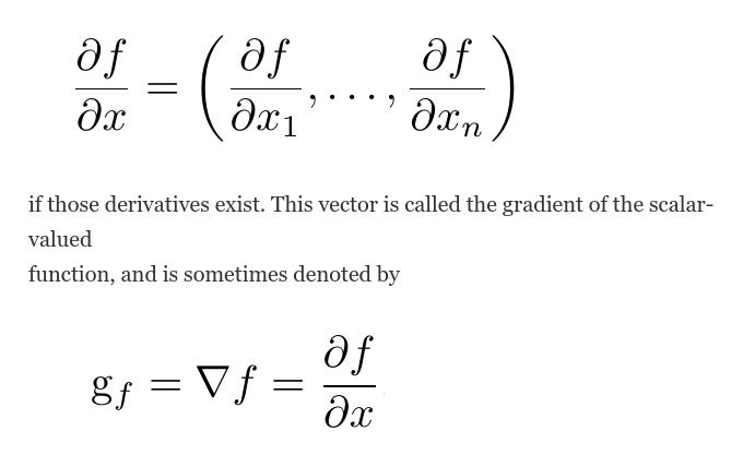
The notation g_f or ∇f implies differentiation with respect to “all” arguments of f , hence, if f is a scalar-valued function of a vector argument, they represent a vector. This derivative is useful in finding the maximum or minimum of a function. Such applications arise throughout statistical and numerical analysis.
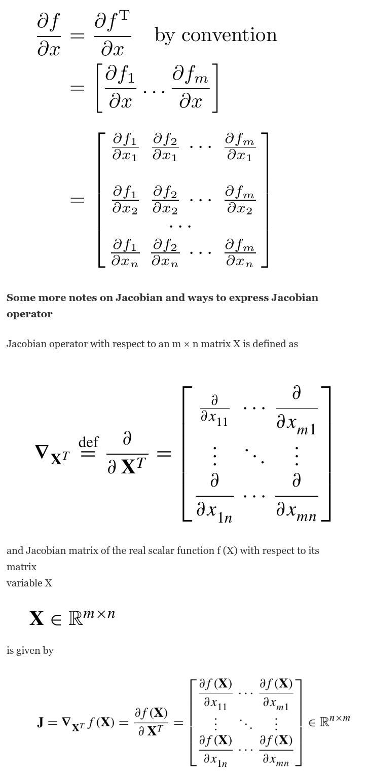
Derivatives of Vectors with Respect to Vectors; The Jacobian
The derivative of an m-vector-valued function of an n-vector argument con- sists of nm scalar derivatives. These derivatives could be put into various structures. Two obvious structures are an n × m matrix and an m × n matrix.
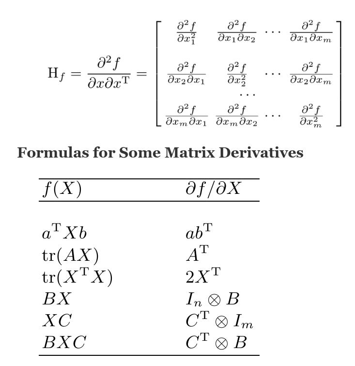
Higher-Order Derivatives with Respect to Vectors; The Hessian
Higher-order derivatives are derivatives of lower-order derivatives. As we have seen, a derivative of a given function with respect to a vector is a more complicated object than the original function. The simplest higher-order derivative with respect to a vector is the second-order derivative of a scalar-valued function. Higher-order derivatives may become uselessly complicated. In accordance with the meaning of derivatives of vectors with respect to vectors, the second derivative of a scalar-valued function with respect to a vector is a matrix of the partial derivatives of the function with respect to the elements of the vector. This matrix is called the Hessian, and is denoted by Hf or sometimes by ∇f or ∇^2f :