
🚀AttentionHead - PyTorch code understanding of a Transformer Architecture🚀🚀
Single Attention Head Pytorch Implementation - Understanding each step

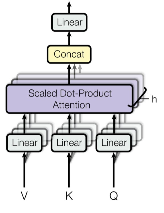
The Attention Layer can be expressed in a single line like below

The PyTorch implementation is below in the Code and lets go-through it line by line.
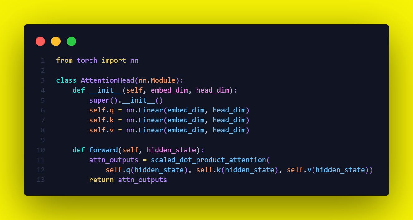
The line `self.q(hidden_state), self.k(hidden_state), self.v(hidden_state))` is performing a linear transformation of the `hidden_state` into query, key, and value components, respectively, for the attention mechanism.
The "hidden_state" here typically refers to the output from the previous layer in the transformer model, and it's usually a 3D tensor with shape `[batch_size, seq_length, embed_dim]`.
▶️ `batch_size`: the number of sequences (or "batches") being processed at once.
▶️ `seq_length`: the number of tokens in each sequence.
▶️ `embed_dim`: the size of the embedding for each token, which is basically a numerical representation of the token's meaning.
Each of the `nn.Linear` objects `(self.q, self.k, self.v)` are layers that will apply a linear transformation to the input. They have their own internal parameters (weights and biases) which are learned during the training process. They are initialized with dimensions `embed_dim x head_dim`.
-----------------
💡What is `hidden_state` in the above context.💡
In the context of transformer models, and deep learning in general, the term "`hidden_state`" typically refers to the intermediate output produced by a layer in the model.
In this case, "hidden_state" is the input to the AttentionHead module, and it would be the output from the previous layer in the transformer model.
A Transformer model consists of several layers, each of which has a self-attention component. The input to each layer (after the first one) is the output from the previous layer. This input is often referred to as the "`hidden_state`" because it's an internal state of the model, representing learned features at that point in the processing of the input.
For the transformer model, the `hidden_state` can be thought of as a representation of the input sequence (a sentence, for instance), but in a higher, more abstract dimensional space, which ideally captures the semantic relationships between the words in the sentence, as well as their syntactic structure.
At the start, the initial "`hidden_state`" is usually just the embeddings of the input sequence. For instance, if you're processing a sentence, you would start with word embeddings for each word in the sentence. The Transformer model then processes these embeddings through several layers, each of which updates this "`hidden_state`" to progressively more abstract representations.
In terms of tensor dimensions, the `hidden_state` is usually a 3D tensor with dimensions [batch_size, sequence_length, embedding_dimension]:
------------------
💡Let's break down the operation `self.q(hidden_state)`.💡
The `nn.Linear(embed_dim, head_dim)` layer is a fully-connected layer that applies a linear transformation to its input, following the formula `y = xA^T + b` where:
▶️ x is the input
▶️ A is the transposed weight matrix inside the layer (self.q.weight)
▶️ b is the bias vector (self.q.bias)
💡💡💡💡 When we call `self.q(hidden_state)`, we're passing the `hidden_state` through this linear layer. Suppose the `hidden_state` has dimensions [batch_size, seq_length, embed_dim]. The linear layer will apply the same transformation to every token of every sequence in the batch (the last dimension), resulting in a new tensor with dimensions [batch_size, seq_length, head_dim].💡💡💡💡
💡💡💡💡The outputs of self.q(hidden_state), self.k(hidden_state), self.v(hidden_state)) are all tensors of shape [batch_size, seq_length, head_dim]. They represent different transformations of the `hidden_state`, corresponding to the query, key, and value used in the attention mechanism. They're then fed into the `scaled_dot_product_attention` function to compute the attention scores and resulting context vectors.
-----------------
💡💡💡💡 Steps of the execution of this line `self.q(hidden_state)`
First note `hidden_state` has dimensions `[batch_size, seq_length, embed_dim]`.
In our case, the linear layer has been initialized with an input size (in_features) equal to embed_dim and output size (out_features) equal to head_dim.
This means the weight matrix A in this layer is of the shape [embed_dim, head_dim].
▶️ Now, when we apply this linear layer to the `hidden_state` using `self.q(hidden_state)`, here's how the computation happens:
▶️ For each token in every sequence of the batch, there is an embedded vector of size embed_dim. This vector represents that token's features. Let's call it x.
▶️ A (the weight matrix of the layer, of size [embed_dim, head_dim]) is multiplied with x (our token's features vector, of size embed_dim). Note that in linear algebra, the product of a vector (of size n) and a matrix (of size n x m) results in a new vector of size m.
▶️ This multiplication is then added to b (the bias vector, of size head_dim).
▶️ The result of above steps is the output y, a vector of size head_dim.
This operation is applied independently to the embedding of every token in every sequence of the batch.
💡 Since the operation is applied to each token in each sequence independently, the first two dimensions of the tensor (batch_size and seq_length) remain unchanged.
💡 Only the size of the last dimension changes from embed_dim to head_dim, because we are transforming each embed_dim-dimensional token embedding into a head_dim-dimensional output.
💡So, if our `hidden_state`'s shape was `[batch_size, seq_length, embed_dim]`, after this linear transformation it becomes `[batch_size, seq_length, head_dim]`.
----------------
💡💡But, how exactly - The weights of the linear layer transform the embed_dim (512 dimensions in our example) to the head_dim (let's say 64 dimensions). 💡💡
Here's how the flow goes
▶️ Initialization: When the linear layer is initialized with `nn.Linear(512, 64)`, PyTorch internally creates a weight matrix of size `[512, 64]` and a bias vector of size [64]. These are the learnable parameters of the layer.
▶️ Input: When we call the linear layer with some input, like `self.q(hidden_state)`, the input data for each token has shape [512] (as per our example). This represents the embed_dim-dimensional embedding of the token.
▶️ Matrix multiplication: The linear layer multiplies the input vector with the transposed weight matrix. Since the input vector is of size [512] and the weight matrix is of size [512, 64], the output of this multiplication is a vector of size [64]. This operation essentially performs a weighted combination of the input features, transforming them into head_dim dimensions.
▶️ Addition of bias: After the matrix multiplication, the layer adds the bias vector to the output. The bias vector is also of size [64], so it can be added element-wise to the output vector. This finalizes the transformation from embed_dim to head_dim.
▶️ So the key point is that the weight matrix acts as a transformation matrix that remaps the input features (embed_dim) to a new space (head_dim).
Let's illustrate with an example. Consider a batch of 8 sequences, each sequence having a length of 10, and an embedding size of 512 (this is a common size in many transformer models). If we assume the dimension of each attention head (head_dim) to be 64, here's how the shapes transform:
▶️ Input hidden_state: [8, 10, 512] # (batch_size, seq_length, embed_dim)
▶️ After transformation (self.q(hidden_state)): [8, 10, 64] # (batch_size, seq_length, head_dim)
▶️ Similarly for self.k(hidden_state) and self.v(hidden_state): [8, 10, 64]
This demonstrates how the Linear layers in the AttentionHead class transform the hidden_state's embeddings into the query, key, and value for the attention mechanism.
Subscribe to to my MachineLearning YouTube channel