Batch Normalization in Deep Learning

Batch normalization was introduced by Google scientists Sergey Ioffe and Christian Szegedy in 2015. Their insight was as simple as it was groundbreaking. Just as we normalize network inputs, they proposed to normalize the inputs to each layer, for each training mini-batch as it flows through the network.

See “Batch Normalization: Accelerating Deep Network Training by Reducing Internal Covariate Shift,” by Sergey Ioffe and Christian Szegedy, 2015, https://arxiv.org/abs/1502.03167.

The Original Problem that Batch Normalization solves

One common challenge when training a deep neural network is ensuring that the weights of the network remain within a reasonable range of values — if they start to become too large, this is a sign that your network is suffering from what is known as the exploding gradient problem. As errors are propagated backward through the network, the calculation of the gradient in the earlier layers can sometimes grow exponentially large, causing wild fluctuations in the weight values. If your loss function starts to return NaN, chances are that your weights have grown large enough to cause an overflow error. This doesn’t necessarily happen immediately as you start training the network. Sometimes your network can be happily training for hours when suddenly the loss function returns NaN and your network has exploded.

Hence, one of the reasons for scaling input data into a neural network is to ensure a stable start to training over the first few iterations. Since the weights of the network are initially randomized, unscaled input could potentially create huge activation values that immediately lead to exploding gradients. For example, instead of passing pixel values from 0–255 into the input layer, we usually scale these values to between –1 and 1.

Because the input is scaled, it’s natural to expect the activations from all future layers to be relatively well scaled as well. Initially, this may be true, but as the network trains and the weights move further away from their random initial values, this assumption can start to break down. This phenomenon is known as covariate shift.

Batch normalization is a solution that drastically reduces this problem. The solution is surprisingly simple. A batch normalization layer calculates the mean and standard deviation of each of its input channels across the batch and normalizes by subtracting the mean and dividing by the standard deviation. There are then two learned parameters for each channel, the scale (gamma) and shift (beta). The output is simply the normalized input, scaled by gamma and shifted by beta.

Understanding normalization

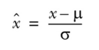
It helps to remind ourselves what normalization is and why we bother normalizing the input feature values in the first place. Normalization is the scaling of data so that it has zero mean and unit variance. This is ccomplished by taking each data point x, subtracting the mean μ, and dividing the result by the standard deviation, σ

Normalization has several advantages. Perhaps most important, it makes comparisons between features with vastly different scales easier and, by extension, makes the training process less sensitive to the scale of the features.

Computing batch normalization

The way batch normalization is computed differs in several respects from the simple normalization equation we presented earlier.

Let μ_B be the mean of the mini-batch B, and σ² be the variance (mean squared deviation) of the mini-batch B. The normalized value is computed as

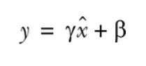
Importantly, the terms γ and β are trainable parameters, which — just like weights and biases — are tuned during network training.

The reason for this is that it may be beneficial for the intermediate input values to be standardized around a mean other than 0 and have a variance other than 1. Because γ and β are trainable, the network can learn what values work best.

Batch normalization limits the amount by which updating the parameters in the previous layers can affect the distribution of inputs received by the current layer. This decreases any unwanted interdependence between parameters across layers, which helps speed up the network training process and increase its robustness, especially when it comes to network parameter initialization.

Quoting from the Original Paper — Batch Normalization: Accelerating Deep Network Training by Reducing Internal Covariate Shift

We define Internal Covariate Shift as the change in the distribution of network activations due to the change in network parameters during training. To improve the training, we seek to reduce the internal covariate shift. By fixing the distribution of the layer inputs x as the training progresses, we expect to improve the training speed. It has been long known (LeCun et al., 1998b; Wiesler & Ney, 2011) that the network training converges faster if its inputs are whitened — i.e., linearly transformed to have zero means and unit variances, and decorrelated. As each layer observes the inputs produced by the layers below, it would be advantageous to achieve the same whitening of the inputs of each layer. By whitening the inputs to each layer, we would take a step towards achieving the fixed distributions of inputs that would remove the ill effects of the internal covariate shift.

Where do I call the BatchNormalization (BN) function in during training a Neural Network ?

There is no correct answer, however, the authors of Batch Normalization say that It should be applied immediately before the non-linearity of the current layer. The reason ( quoted from original paper) -

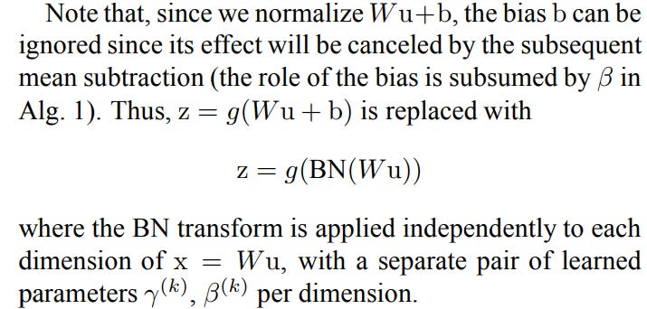
“We add the BN transform immediately before the nonlinearity, by normalizing x = Wu+b. We could have also normalized the layer inputs u, but since u is likely the output of another nonlinearity, the shape of its distribution is likely to change during training, and constraining its first and second moments would not eliminate the covariate shift. In contrast, Wu + b is more likely to have a symmetric, non-sparse distribution, that is “more Gaussian” (Hyv¨arinen & Oja, 2000); normalizing it is likely to produce activations with a stable distribution.”

So from the paper equation is g(BN(Wx + b)) , where g is the activation function.

Batch Normalization is just another layer, so you can use it as such to create your desired network architecture. There are reports of models getting better results when using batch normalization after the activation, while others get best results when the batch normalization is placed before the activation. It is probably best to test your model using both configurations, and if batch normalization after activation gives a significant decrease in validation loss, use that configuration instead.

Many suggest BN should go between the linear transform and nonlinearity is the right place for the normalization, because it normalizes the input to your activation function, so that you’re centered in the linear section of the activation function (such as Sigmoid).

So the following Keras code is a very standard classic application of BN following the above (i.e. BN before Activation )

from keras.layers.normalization import BatchNormalization
# instantiate model
model = Sequential()
# we can think of this chunk as the input layer
model.add(Dense(64, input_dim=14, init='uniform'))
model.add(BatchNormalization())
model.add(Activation('tanh'))
model.add(Dropout(0.5))

# we can think of this chunk as the hidden layer
model.add(Dense(64, init='uniform'))
model.add(BatchNormalization())
model.add(Activation('tanh'))
model.add(Dropout(0.5))

# we can think of this chunk as the output layer
model.add(Dense(2, init='uniform'))
model.add(BatchNormalization())
model.add(Activation('softmax'))
# setting up the optimization of our weights
sgd = SGD(lr=0.1, decay=1e-6, momentum=0.9, nesterov=True)
model.compile(loss='binary_crossentropy', optimizer=sgd)
# running the fitting
model.fit(X_train, y_train, nb_epoch=20, batch_size=16, show_accuracy=True, validation_split=0.2, verbose = 2)

But on the other hand many have suggested Batch normalization works best after the activation function. And their logic goes this way — That BN was developed to prevent internal covariate shift. Internal covariate shift occurs when the distribution of the activations of a layer shifts significantly throughout training, because of parameter updates and this slows the learning.

So Batch normalization is used so that the distribution of the inputs (and these inputs are literally the result of an activation function) to a specific layer doesn’t change over time due to parameter updates from each batch (or at least, allows it to change in an advantageous way).

It uses batch statistics to do the normalizing, and then uses the batch normalization parameters (gamma and beta in the original paper) “to make sure that the transformation inserted in the network can represent the identity transform” (quote from original paper). But the point is that we’re trying to normalize the inputs to a layer, so it should always go immediately before the next layer in the network. Whether or not that’s after an activation function is dependent on the architecture in question.

Batch Normalization in Keras Source Code

keras.layers.BatchNormalization handles all the mini-batch computations and updates behind the scenes for us.

As per its documents — Batch normalization applies a transformation that maintains the mean output close to 0 and the output standard deviation close to 1.

If you are interested you can take a look at this Keras implementaion of Batch Normalization Code

---

Overall The benefits of batch normalization are as follows:

Reduces the internal covariate shift: Batch normalization helps us to reduce the internal covariate shift by normalizing values.

Faster training: Networks will be trained faster if the values are sampled from a normal/Gaussian distribution. Batch normalization helps to whiten the values to the internal layers of our network. The overall training is faster, but each iteration slows down due to the fact that extra calculations are involved.

Higher accuracy: Batch normalization provides better accuracy.

Higher learning rate: Generally, when we train neural networks, we use a lower learning rate, which takes a long time to converge the network. But with BN, because of the normalizing effect with additional layer in deep neural networks, the network can use higher learning rate without vanishing or exploding gradients, making our network reach the global minimum faster.

Reduces the need for dropout: When we use dropout, we compromise some of the essential information in the internal layers of the network. Batch normalization acts as a regularizer, meaning we can train the network without a dropout layer. Batch normalization also has been shown to reduce overfitting, and therefore many modern deep learning architectures don’t use dropout at all, and rely solely on batch normalization for regularization.

As with most deep learning principles, there is no golden rule that applies in every situation — the only way to know for sure what’s best is to test different architectures and see which performs best on a holdout set of data.