Bias-Variance Trade-off in DataScience and Calculating with Python

The target of this blog post is to discuss the concept around and the Mathematics behind the below formulation of Bias-Variance Tradeoff.

And in super simple term

Total Prediction Error = Bias + Variance

The goal of any supervised machine learning model is to best estimate the mapping function (f) for the output/dependent variable (Y) given the input/independent variable (X). The mapping function is often called the target function because it is the function that a given supervised machine learning algorithm aims to approximate.

The Expected Prediction Error for any machine learning algorithm can be broken down into three parts:

Bias Error Variance Error Irreducible Error

Why at all we need for MSE (Mean Squared Error) for training and testing datasets separately

Exploring these in detail is very important to understand the whole concepts around the Bias-Variance tradeoff.

Training and testing datasets have different purposes.

The training set trains the model how to predict the dependent variable values and we derive the Estimator equation from the training dataset. While, the testing datasets are there for testing the Estimator equation on how good an estimator they are really.

Now lets examine this in depth.

In the regression setting, the most commonly-used measure is the mean squared error (MSE), is given by

where f ˆ (x i) is the prediction that f ˆ gives for the i-th observation. The MSE will be small if the predicted responses are very close to the true responses, and will be large if for some of the observations, the predicted and true responses differ substantially. The Test-MSE Equation is computed using the training data that was used to fit the model, and so should more accurately be referred to as the training MSE. But in general, we do not really care how well the method works training on the training data. Rather, we are interested in the accuracy of the predictions that we obtain when we apply our method to previously unseen test data.

Why is this what we care about? Suppose that we are interested test data in developing an algorithm to predict a stock’s price based on previous stock returns. We can train the method using stock returns from the past 6 months. But we don’t really care how well our method predicts last week’s stock price. We instead care about how well it will predict tomorrow’s price or next month’s price.

To state it more mathematically, suppose that we fit our statistical learn- ing method on our training observations {(x1 , y 1 ), (x2 , y2 ), . . . , (xn , yn)}, and we obtain the estimated f̂. We can then compute

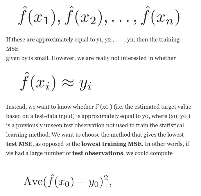
the average squared prediction error for these test observations (x0 , y0 ). And then we’d just like to select the model for which the average of this quantity — the test MSE — is as small as possible.

But what if no test observations are available? In that case, one might imagine simply selecting a statistical learning method that minimizes the training MSE. Unfortunately, this strategy does not work. There is no guarantee that the method with the lowest training MSE will also have the lowest test MSE.

The below figure-A illustrates this phenomenon on a simple example.

In the lefthand panel of Figure A, we have generated observations from  true f given by the black curve. The orange, blue and green curves illus- trate three possible estimates for f obtained using methods with increasing levels of flexibility. The orange line is the linear regression fit, which is relatively inflexible. The blue and green curves were produced using smoothing splines. It is clear that as the level of flexibility increases, the curves fit the observed data more closely.

We now move on to the right-hand panel of Figure-A. The grey curve displays the average training MSE as a function of flexibility, or more formally the degrees of freedom, for a number of smoothing splines. The degrees of freedom is a quantity that summarizes the flexibility of a curve.

The test MSE is displayed using the red curve in the right-hand panel of Figure A. As with the training MSE, the test MSE initially declines as the level of flexibility increases. However, at some point the test MSE levels off and then starts to increase again. Consequently, the orange and green curves both have high test MSE. The blue curve minimizes the test MSE, which should not be surprising given that visually it appears to estimate f the best in the lefthand panel of Figure-A

In the right-hand panel of Figure-A, as the flexibility of the statistical learning method increases, we observe a monotone decrease in the training MSE and a U-shape in the test MSE. This is a fundamental property of statistical learning that holds regardless of the particular data set at hand and regardless of the statistical method being used.

As model flexibility increases, training MSE will decrease, but the test MSE may not.

And when a given method yields a small training MSE but a large test MSE, we are said to be overfitting the data. This happens because our statistical learning procedure is working too hard to find patterns in the training data, and maybe picking up some patterns that are just caused by random chance rather than by true properties of the unknown function f.

However, regardless of whether or not overfitting has occurred, we almost always expect the training MSE to be smaller than the test MSE because most statistical learning methods either directly or indirectly seek to minimize the training MSE.

So now the final point which is The Bias-Variance Trade-Off

The U-shape observed in the test MSE curves in Figure-A above turns out to be the result of two competing properties of statistical learning methods. It is possible to show that the **expected test MSE (**or sometimes also called Expected Prediction Error ), for a given value x0, can always be decomposed into the sum of three fundamental quantities: the variance of estimated f(x0 ), the squared bias of estimated f(x0 ) and the variance of the error terms.

The left-hand side of the above equation defines the expected test MSE and refers to the average test MSE that we would obtain if we repeatedly estimated f using a large number of training sets, and tested each at x0. The overall expected test MSE can be computed by averaging over all possible values of x0 in the test set

Definition of Variance

The variance of the model is the amount the performance of the model changes or the amount by which the estimated f would change, when it is fit on different training data sets. It captures the impact of the specifics the data has on the model.

Since the training data are used to fit the statistical learning method, different training data sets will result in a different estimated-f . But ideally, the estimate for f should not vary too much between training sets. However, if a method has high variance then small changes in the training data can result in large changes in estimated-f . In general, more flexible statistical methods have higher variance.

Variance informally means how far your data is spread out. Overfitting is you memorizing 10 questions for your exam and on the next day exam, only one question (our of that 10 memorized) has been asked in the question paper. Now you will answer that one question correctly (based on training), but you have no idea what the remaining questions are(Question are HIGHLY VARIED from what you read). In overfitting, the model will memorize the entire train data such that it will give high accuracy on the training-dataset but will fail in test.

For high variance models an alternative is feature reduction (e.g. pruning in Decision Tree, we will cover this in more detail further down in this article), but including more training data is also a viable option. This means when I repeat the entire model building process multiple times, the variance is HOW MUCH THE PREDICTIONS FOR A GIVEN POINT VARY, between different realizations of the model.

Let θ̂ be a point estimator for a parameter θ

Definition of Bias

bias refers to the error that is introduced by approximating a real-life problem, which may be extremely complicated, by a much simpler model. For example, linear regression assumes that there is a linear relationship between Y and X1, X2, . . . , Xp . It is unlikely that any real-life problem truly has such a simple linear relationship, and so performing linear regression will undoubtedly result in some bias in the estimate of the f.

In the above figure, the true f is substantially non-linear, so no matter how many training observations we are given, it will not be possible to produce an accurate estimate using linear regression. In other words, linear regression results in high bias in this example.

So, the bias is a measure of how close the model can capture the mapping function between inputs and outputs. When a model has a high bias it means that it is very simple and that adding more features should improve it. Bias does not depend on data

So, the error due to bias is taken as the difference between the expected (or average) prediction value from my model and the correct value which I am trying to predict.

Now the basic question is I am only taking one model so how the concept of expected or average prediction values comes here. To understand that, imagine repeating the whole model building process more than once: each time I gather new data and run a new analysis creating a new model. Due to randomness in the underlying data sets, the resulting models will have a range of predictions. So now, the Bias measures how far off these models’ predictions are from the correct value.

So, let θ̂ be a point estimator for a parameter θ. Then θ̂ is an unbiased estimator if E(θ̂ ) = θ, else θ̂ is said to be biased.

The bias of a point estimator θ̂ is given by

Where, just like the alternate expression of Variance, L=100 data sets each with each with N=25

Actual Calculation of Bias

To find the bias of a model (or method), perform many estimates, and add up the errors in each estimate compared to the real value. Dividing by the number of estimates gives the bias of the method. In statistics, there may be many estimates to find a single value. Bias is the difference between the mean of these estimates and the actual value.

High Bias

The two main reasons for high bias are insufficient model capacity and underfitting because the training phase wasn’t complete. For example, if you have a very complex problem to solve (e.g. image recognition) and you use a model of low capacity (e.g. linear regression) this model would have a high bias as a result of the model not being able to grasp the complexity of the problem.

What is an estimator

An estimator is a rule, often expressed as a formula, that tells how to calculate the value of an estimate based on the measurements contained in a sample.

For example, the sample mean

is one possible point estimator of the population mean μ. Clearly, the expression for ȳ is both a rule and a formula. It tells us to sum the sample observations and divide by the sample size n.

In machine learning, an estimator is an equation for picking the “best,” or most likely accurate, data model based upon observations in realty. Not to be confused with estimation in general, the estimator is the formula that evaluates a given quantity (the estimand) and generates an estimate (source).

Now lets see the process of calculating Estimates

Suppose that we wish to specify a point estimate for a population parameter that we will call θ . The estimator of θ will be indicated by the symbol θ̂, read as “θ hat.” The “hat” indicates that we are estimating the parameter immediately beneath it. We can say that it is highly desirable for the distribution of estimates — or, more properly, the sampling distribution (where Learning Samples are randomly drawn) of the estimator — to cluster about the target parameter as shown in Figure-A. In other words, we would like the mean or expected value of the distribution of estimates to equal the parameter estimated; that is, E(θ̂) = θ. Point estimators that satisfy this property are said to be unbiased.

The sampling distribution for a positively biased point estimator, one for which E(θ̂) > θ , is shown in Figure-B.

Figure-C below shows two possible sampling distributions for unbiased point estimators for a target parameter θ. We would prefer that our estimator have the type of distribution indicated in Figure C-(b) because the smaller variance guarantees that in repeated sampling a higher fraction of values of θ̂ 2 will be “close” to θ. Thus, in addition to preferring unbiasedness, we want the variance of the distribution of the estimator V (θ̂ ) to be as small as possible. Given two unbiased estimators of a parameter θ, and all other things being equal, we would select the estimator with the smaller variance.

Below a very popular graph, you will see in many pieces of literature describing the relationship between Bias and Variance.

Some Interpretations from the above Graph

Looking at the above plot, some observations we can see, that the bias tends to decrease faster than the variance increases. So when tuning our model, this portion of the curve, is like the low-hanging fruit that we can easily get — so an incremental improvement on the red curve above gives a big decrease in bias (increase in performance). However, when we continue further on this path, with each increment in model complexity, you get a lower increase in performance; i.e. diminishing returns sets in. Furthermore, as you begin to overfit, the model becomes less able to generalize and so exhibits larger errors on unseen data i.e . Variance is creeping in.

The key Equation of Variance and Bias

The mean square error of an estimator θ̂ , MSE(θ̂), is a function of both its variance and its bias. If B(θ̂ ) denotes the bias of the estimator θ̂ the relation between them can be expressed as (we will go through the proof of this below)

MSE(θ̂) = V(θ̂) + [B(θ̂)]²

Which more generally will be below

Bias Variance Tradeoff

There is no escape from the relationship between bias and variance in machine learning which in general is

• Increasing the bias will decrease the variance.

• Increasing the variance will decrease the bias.

In short, the bias is the model’s inability to learn enough about the relationship between the model’s features and labels, while the variance captures the model’s inability to generalize on new, unseen examples. A model with high bias oversimplifies the relationship and is said to be underfit. A model with high variance has learned too much about the training data and is said to be overfit. Of course, the goal of any ML model is to have low bias and low variance but, in practice, it is hard to achieve both. For example, increasing model complexity decreases bias but increases variance, while decreasing model complexity decreases variance but introduces more bias.

However, recent work suggests that when using modern machine learning techniques such as large neural networks with high capacity, this behavior is valid only up to a point. In observed experiments, there is an “interpolation threshold” beyond which very high capacity models are able to achieve zero training error as well as low error on unseen data. Of course, you need much larger datasets in order to avoid overfitting on high capacity models.

The Tradeoff in a Nutshell

• A model with low variance and low bias is the ideal model.

• A model with low bias and high variance is a model with overfitting. Generally speaking, overfitting means bad generalization, memorization of the training set rather than learning a generic concepts behind the data.

• A model with high bias and low variance is usually an underfitting model.

• A model with high bias and high variance is the worst case scenario, as it is a model that produces the greatest possible prediction error.

Mathematical Derivation of the Bias-Variance Equation

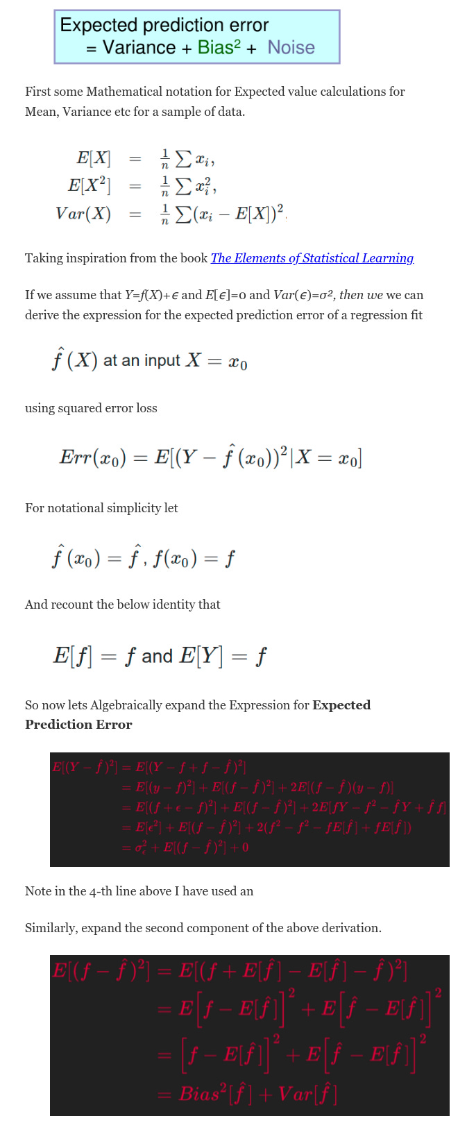
Combining from the above two derivations we get the final relation between Expected Prediction Error on the LHS and the Bias and Variance of the estimator as below.

Ways to mitigate this bias-variance tradeoff on small- and medium- scale problems

Ensemble methods to the rescue, which are meta-algorithms which combine several machine learning models as a technique to decrease the bias and/or variance and improve model performance.

Instead of fitting a single final model, you can fit multiple final models. Together, the group of final models may be used as an ensemble. For a given input, each model in the ensemble makes a prediction and the final output prediction is taken as the average of the predictions of the models.

By building several models, with different inductive biases, and aggregating their outputs, we hope to get a model with better performance. Below, we’ll discuss some commonly used Ensemble methods, including bagging, boosting, and stacking.

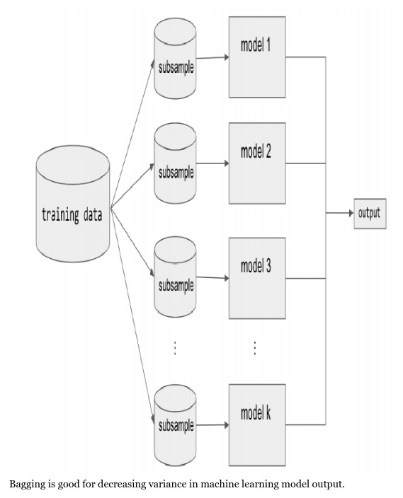
BAGGING

Bagging (short for bootstrap aggregating) is a type of parallel ensembling method and it is used to address high-variance in machine learning models. The bootstrap part of bagging refers to the datasets used for training the ensemble members. Specifically, if there are k sub-model then there are k separate datasets used for training each sub-model of the ensemble. Each dataset is constructed by randomly sampling (with replacement) from the original training dataset. This means there is a high probability that any of the k datasets will be missing some training examples, but also any dataset will likely have repeated training examples. The aggregation takes place on the output of the multiple ensemble model members, either an average in the case of a regression task or a majority vote in the case of classification. A good example of a bagging Ensemble method is the Random Forest: multiple decision trees are trained on randomly sampled subsets of the entire training data, then the tree predictions are aggregated to produce a prediction, as shown in below Figure.

Most recognized machine learning libraries have implementations of bagging methods. For example, to implement a Random Forest regression in scikit-learn

from sklearn.ensemble import RandomForestRegressor
# Create the model with 50 trees
RF_model = RandomForestRegressor(n_estimators=50,
max_features='sqrt',
n_jobs=-1, verbose = 1)
# Fit on training data
RF_model.fit(X_train, Y_train)

Model averaging as seen in bagging is a powerful and reliable method for reducing model variance. Different Ensemble methods combine multiple sub-models in different ways, sometimes using different models, different algorithms, or even different objective functions. With bagging, the model and algorithms are the same. For example, with Random Forest, the submodels are all short Decision Trees.

The next Ensemble technique is BOOSTING Unlike bagging, boosting ultimately constructs an ensemble model with more capacity than the individual member models. For this reason, boosting provides a more effective means of reducing bias than variance. The idea behind boosting is to iteratively build an Ensemble of models where each successive model focuses on learning the examples the previous model got wrong. In short, boosting iteratively improves upon a sequence of weak learners taking a weighted average to ultimately yield a strong learner.

The next Ensemble technique is STACKING Stacking is an Ensemble method which combines the outputs of a collection of models to make a prediction. The initial models, which are typically of different model types, are trained to completion on the full training dataset. Then, a secondary meta-model is trained using the initial model outputs as features. This second meta-model learns how to best combine the outcomes of the initial models to decrease the training error and can be any type of machine learning model.

An example of reducing Variance of a Decision Tree

Decision trees are powerful classifiers. Algorithms such as Bagging try to use powerful classifiers in order to achieve ensemble learning for finding a classifier that does not have high variance. But Decision trees are prone to overfitting. A model has high variance if it is very sensitive to (small) changes in the training data. Models that exhibit overfitting are usually non-linear and have low bias and variance . Decision trees are non-linear.

A decision tree has high variance because, if you imagine a very large tree, it can basically adjust its predictions to every single input.

Consider you wanted to predict the outcome of a Cricket game. A decision tree could make decisions like:

IF

1. player X is on the field AND

2. team A has a won the toss AND

3. the weather is sunny AND

4. the number of attending fans >= 26000 AND

5. it is past 3pm

THEN team A wins.

If the tree is very deep, it will get very specific and you may only have one such game in your training data. It probably would not be reasonable to base your predictions on just one example.

Now, if you make a small change e.g. set the number of attending fans to 25999, a decision tree might give you a completely different answer (because the game now doesn’t meet the 4th condition).

Linear regression, for example, would not be so sensitive to a small change because it is limited (or “biased” ) to linear relationships and cannot represent sudden changes from 25999 to 26000 fans.

That’s why it is important to not make decision trees arbitrary large/deep. This limits its variance.

This is why we usually use pruning for avoiding the trees to get overfitted to the training data. Pruning reduces the size of decision trees by removing parts of the tree that do not provide power to classify instances. One way can be ignoring some features and using others. Pruning is computationally inexpensive, reduces complexity significantly, and variance to some extent, but also increases bias.

Thank you for reading :)