
Concepts of Differential Calculus for understanding Gradient Descent
Application in Linear Regression

What Derivative of a function really is

What Derivative of a function really is
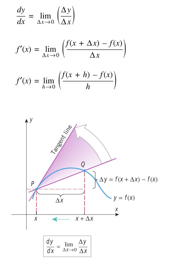
The most fundamental defination of Derivative can be stated as — derivative measures the steepness of the graph of a function at some particular point on the graph. Thus, the derivative of a function is a slope at a particular point. Strictly speaking, curves don’t have slope, so we use the slope of the tangent line at a particular point on the curve. That also means that it is a ratio of change in the value of the function (dependent variable) to the change in the independent variable.
Take a note in the above image, when Δx approaches 0, the secant line become Tangent at x0 and derivative of the function representing the above graph gives the slope of the tangent line at x0.
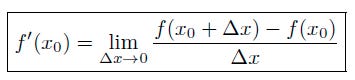
So we define the derivative of the function f(x) at the point x0, as the limit of the the slope as Δx approaches zero:
One of the essential idea in differential calculus is about approximating non-linear objects by linear ones. And we already saw, that a tangent line at a point is the best linear approximation to the curve near that point.
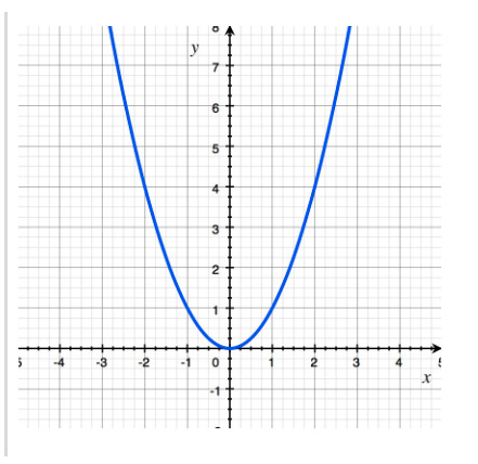
Now quickly visualize the above concept — We will see later that by the rules of Differential Calculus (Power Rule) “The derivative of x² is 2x” which means “At every point, we are changing by a speed of 2x (twice the current x-position)”.
And below is the graph of a function f(x) = x². As you can see just looking at the graph y is changing at double the rate of x. Which is what derivative measures.
Derivative can also be intutively understood as representing rate of change.
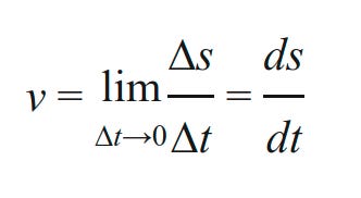
Take the most simplest real world example of Velocity, which is defined as the rate of change of displacement with respect to time. And Displacement here is a function of time and the dependent variable and the independent variable is “time”. Now t_he_ function has been plotted on a graph. And now we’ll see that the concept of velocity and slope of a curve are connected by the same mathematical definition.
Now Velocity is the change in displacement, and so we can think of the ratio as a rate of change of displacement with the rate of change of time to be the derivative of the time function and is called the Velocity.
A derivative of a function is a representation of the rate of change of one variable in relation to another at a given point on a function. The slope describes the steepness of a line as a relationship between the change in y-values for a change in the x-values. However note, afunction does not have a general slope. We cannot have a slope of y = x² at x = 2**, instead what we can have is the slope of the line tangent to this point.**
The first-principle defination of Derivative
The derivative of the function y = f (x) with respect to the variable x is the function f′(x) is given by
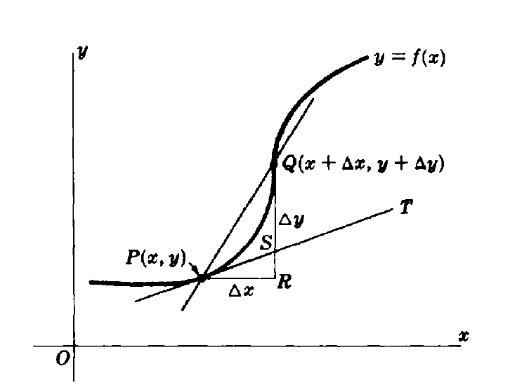
From the above figure we can see that the above derivative formulae expresses the slope of the tangent line as a limit of slopes of secant lines. The slope of a secant line (line connecting two points on a graph) approaches the derivative when the interval between the points shrinks down to zero.
The function f′(x) is called the derivative of f, since it is derived from f by the limiting operation. You can think of f′(x) as a “slope-producing function” in the sense that the value of f′(x) at x = x0 is the slope of the tangent line to the graph of f at x = x0 .
So, from the above, the rules to find out the differentiation by the first principle will be as follows
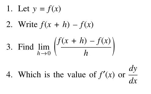
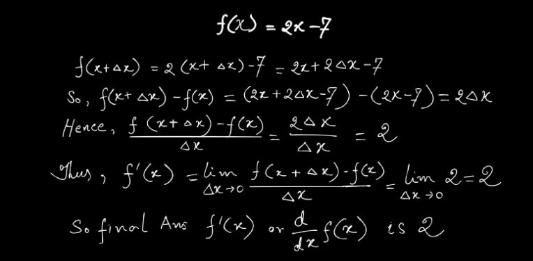
Lets do an example of calculation derivative from first principle
Using the A-definition, find the derivative f′(x) of the function f(x) = 2x — 7
Interpret dy/dx geometrically
From below figure we see that Δ_y_/Δ_x_ is the slope of the secant line joining an arbitrary but fixed point P( x , y ) and a nearby point Q (x+Δ_x_, y+Δ_y_) of the curve.
As Δ_x_ approaches 0, P remains fixed while Q moves along the curve toward P, and the line PQ revolves about P toward its limiting position, the tangent line PT to the curve at P. Thus, dy/dx gives the slope of the tangent at P to the curve y = f ( x )y=f(x) .
Now here’s the most important fundamental Differential Calculus rules that we will need to understand the derivation of the Gradient Descent formulae
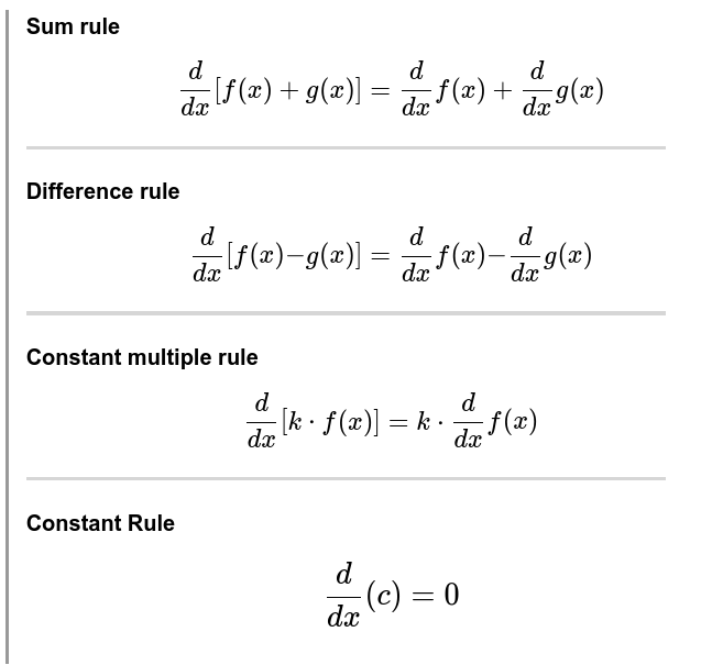
So overall in a nutshell
The Sum rule is almost like a regular arithmatic sum — the derivative of a sum of functions is the sum of their derivatives.
The Difference rule, again just like regular arithmatic says the derivative of a difference of functions is the difference of their derivatives.
The Constant multiple rule says the derivative of a constant multiplied by a function is the constant multiplied by the derivative of the function.
The Constant rule says that the derivative of a constant function is zero; that is, since a constant function is a horizontal line, the slope, or the rate of change, of a constant function is 0
Now lets see some basic implementation of the above differentiation rules that we just learned ?
You can find the derivatives of functions that are combinations of other, simpler, functions. For example lets take a function F(x) which is defined as
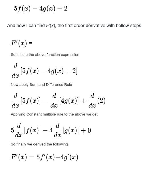
Now for a specific value of x say 2, if we derive that f′(2)=6 and g′(2)=9
Then, we can calculate H′(3) as follows
H′(2)=5_f_′(2)−4_g_′(2)
which is 9–6 ie. -3
Now, beyond the above discussed Sum and Difference rules we also need to take note of the following Differentiation Rules while getting into Linear Regression.
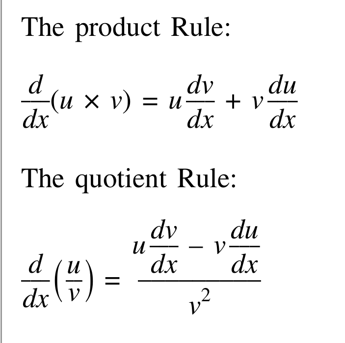
And the all important Chain Rules while dealing with Differentiation of Composite function
First lets see an example of composite function
If f(x) = x² + 2x — 5 and g(x) = x³, find formulas for the composite functions f of g and g of f.
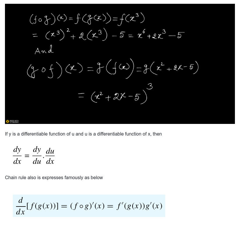
A convenient way to remember the above Chain rule formula is to call f the “outside function” and g the “inside function” in the composition f(g(x)) and then executing the rule as below.
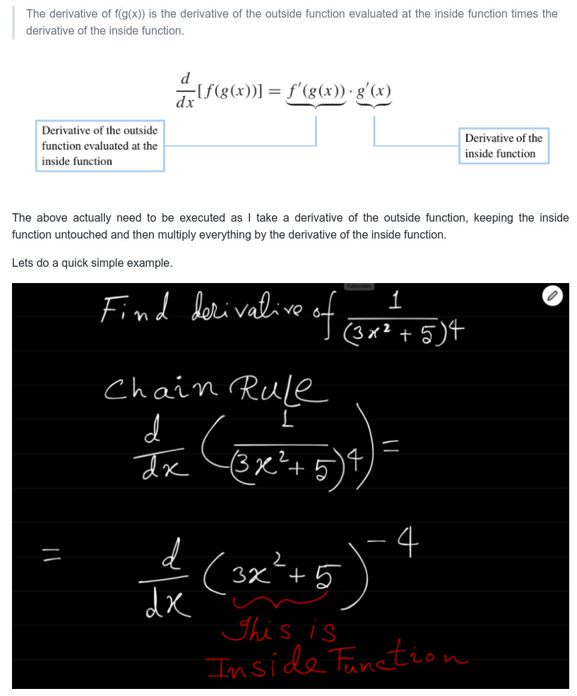
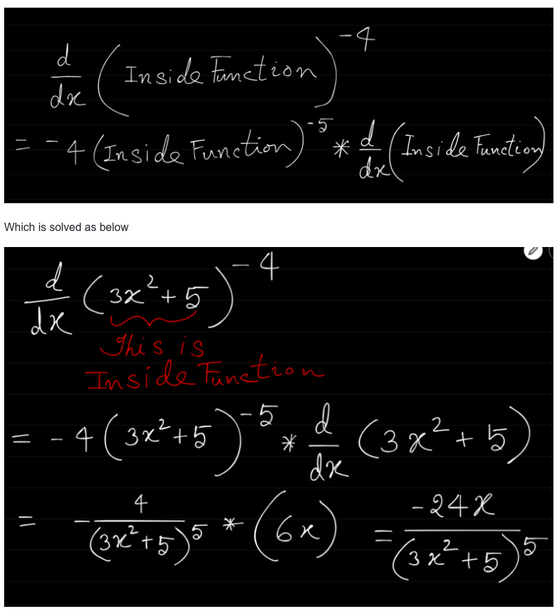
So following the Chain Rule formulae — the above will become of the below form after applying Power Rule of Derivative
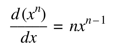
The Power Rule
Is all function differentiable at every point in its graph ?
The ans is NO
So, what does it mean when we say, function f(x) is differentiable at the point x=0
A differentiable function of one real variable is a function whose derivative exists at each point in its domain. As a result, the graph of a differentiable function must have a non-vertical tangent line at each point in its domain, be relatively smooth, and cannot contain any breaks, bends, or cusps.
For example, the absolute value function
f(x)=∣_x_∣
has a sharp graph at the point x=0 , or if its graph has an “infinite slope” near some point, then we should not expect a derivative to be defined there.
So in a nutshell we have following cases for differentiability or not
1. A function f(x) is differentiable in its domain if it is a smooth curve, like the below one.
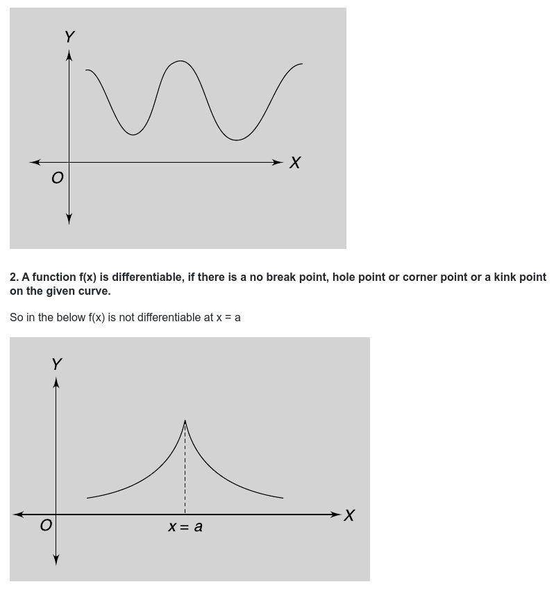
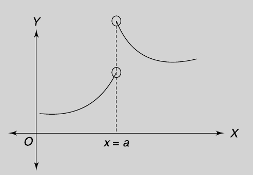
Also in the below f(x) is not differentiable at x = a
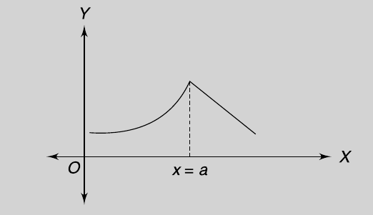
And in the below too, f(x) is not differentiable at x = a
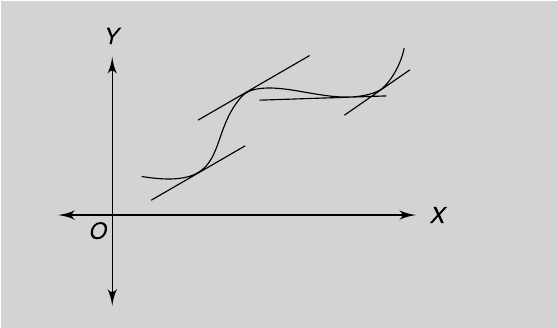
3. A function f(x) is differentiable if there exists a unique tangent to each point on the given curve.
Now note, for fitting a model to the observed data, there are quite few techniques or algorithms, e.g. closed-form equations vs. Gradient Descent vs Stochastic Gradient Descent vs Mini-Batch Learning.
Gradient Descent is probably one of the most fine-tuned one among them.
Gradient Descent Algorithm — The key steps in a nutshell
Initialize the value of coefficients (_θ_0 and _θ_1) randomly.
Calculate the cost function (Mean Squared Error or MSE in short) — that is, the sum of squared error across all the data points in the training dataset. (The Mathematical form below which we will explore in more detail further down)
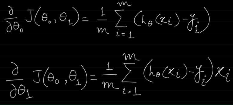
We identify parameters, (θ0 and θ1 ) in the regression function and we take partial derivatives of MSE with respect to these parameters. Each derived function can tell which way we should tune parameters and by how much.
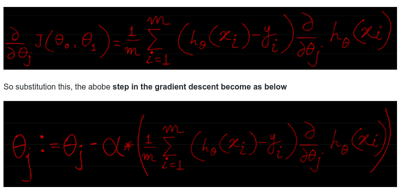
The derivative of this with respect to any weight is the below (this formula shows the gradient computation for linear regression):
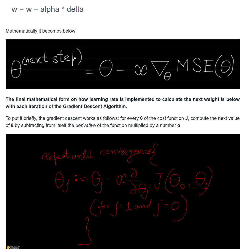
Change the value of coefficients (theta (θ) values in the above Cost function equation) slightly, say, +1% of its value. This % by which the Coeffiecients are changed for next iteration is called Learning Rate.
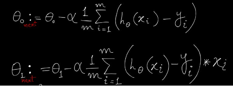
Below is the equation which is applied to get the next Coefficient (theta/θ) . (we will derive this equation from MSE shortly)
The above is what summarizes the Gradient-Descent(GD) Algorithm, which in a nutshell state the below.
The gradient points in the direction of the largest rate of increase of the function, and its magnitude is the slope in that direction. And by the GD-algorithm, if we are at a particular value of θ (representing coefficients of the Linear Regression function) and if we want to move to a new value of θ such that the new loss is less than the current loss then we should move in the direction opposite to the gradient.
Now calculate MSE again and check whether, by changing the value of coefficients (Theta/θ values ) slightly, overall squared error (Mean Squared Error or MSE) decreases or increases.
If overall squared error (MSE) decreases by changing the value of coefficient by +1%, then proceed further in that direction and increase the Coefficient by 1% again. Else, if the MSE increased, then for the next iteration go in the opposite direction i.e. reduce the coefficient by 1%.
Repeat steps 2–6 until overall squared error is the least.
From the above, we can tell that, we’re computing dJ/dTheta-j(the gradient of weight Theta-j) and then we’re taking a step of size alpha in that direction. Hence, we’re moving down the gradient.
How exactly the Minimization is achieved during Gradient Descent by taking Derivative of the Cost the function
To understand that first we have to know how Derivative calculates maximum and minimum values of a function.
Maxima and Minima
For a given dataset, whenever there is a peak in the data, this is a maximum The global maximum is the highest peak in the entire data set, or the largest f(x) value the function can output A local maximum is any peak, when the rate of change switches from positive to negative.
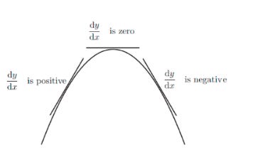
And whenever there is a trough in the data, this is a minimum. The global minimum is the lowest trough in the entire data set, or the smallest f(x) value the function can output A local minimum is any trough, when the rate of change switches from negative to positive.
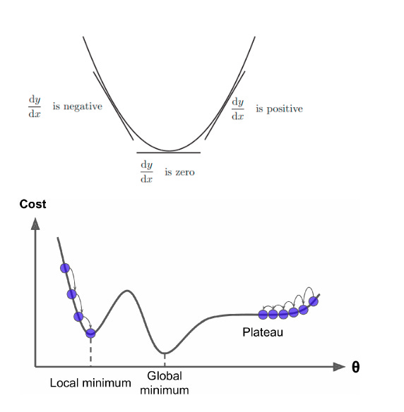
And the key point to remember is — The derivative is zero at any local maximum or minimum. So, one way to find a minimum: set f′(x)=0 and solve for x.
Fortunately, the MSE (Mean Squared Error) cost function for a Linear Regression model happens to be a convex function, which means that if you pick any two points on the curve, the line segment joining them never crosses the curve. This implies that there are no local minima, just one global minimum. It is also a continuous function with a slope that never changes abruptly. These two facts have a great consequence: Gradient Descent is guaranteed to approach arbitrarily close the global minimum (if you wait long enough and if the learning rate is not too high).
In the case of non-linear neural networks, the loss function is typically non-convex, which requires extra techniques during training.
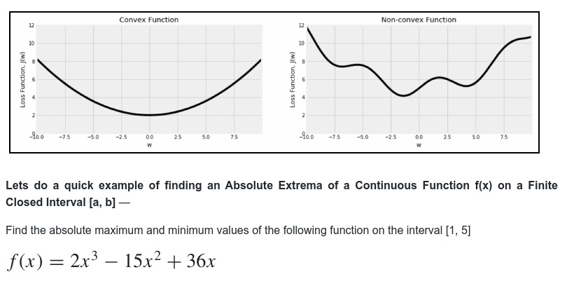
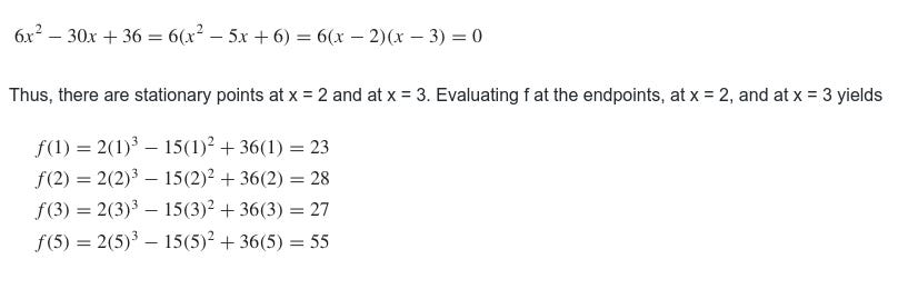
Since f is continuous and differentiable everywhere, the absolute extrema must occur either at endpoints of the interval or at solutions to the equation
f′(x)= 0
in the open interval (1, 5). The equation f′(x) = 0 can be written as
Rules of Increasing and Decreasing function to minimalize cost function and how to decide which way to change the next iteration value of the coefficients (i.e. to increase or to decrease) to arrive at the minimal value of the Cost funtion.
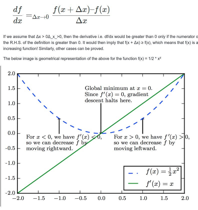
1. For a function f(x), if the first order derivative f′(x) > 0 at each point in an interval (a,b), then the function is said to be a increasing function in (a,b)
So, during the Gradient-Descent algorithm, to determine the direction of the next iteration, for an increasing function don’t move in that direction, because in that case I will be moving away from a trough. In other words, we can decrease f by moving in the direction of the negative gradient.
2. If the first order derivative f′(x) < 0 at each point in an interval (a,b) then the function is said to be decreasing (a,b)
So in this case during Gradient-Descent algorithm, keep moving in this direction, since I am getting closer to a trough
To understand the concept of increasing and decreasing function intuitively think it like this — because we know the derivative is zero or does not exist only at critical points of the function, for all other points where the function exists, it must be positive or negative.
A continuous function f has a local maximum at point c if and only if f switches from increasing to decreasing at point c. Similarly, f has a local minimum at c if and only if f switches from decreasing to increasing at c.
If f′(x)changes sign from positive when xc, then f(c) is a local maximum of f.
If f′(x)changes sign from negative when xc, then f(c) is a local minimum of f.
If f′(x) has the same sign for xc, then f(c) is neither a local maximum nor a local minimum of f.
Proof of the Increasing/Decreasing function
Remember the definition of the derivative of a function:
Gradient Descent
Gradient descent is an optimization algorithm that aims to find a local minimum in a function by iteratively moving in the direction of steepest descent. The direction of the steepest descent is found using calculus, hence the term gradient. If you imagine the objective (loss) function as a curve, the gradient descent algorithm blindly lands on a random point on this curve and uses the gradient at the point it is on as a guiding stick to move to a local minimum step by step. Usually, the loss function is chosen to be a convex one so that its local minima is also its global one.
Mathematically deriving the Gradient Descent from Mean Squared Error (MSE) function
Lets say our Hypothesis function for Linear Regression is as below:
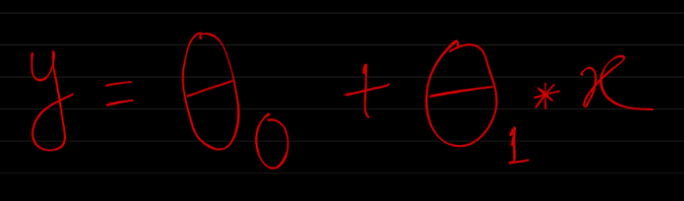
Where,
x: input training data (univariate — one input variable(parameter)) y: labels to data (supervised learning)
During training, it fits the best line to predict the value of y for a given value of x. The model gets the best regression fit line by finding the best θ0 and θ1 values. θ0: intercept θ1: coefficient of x
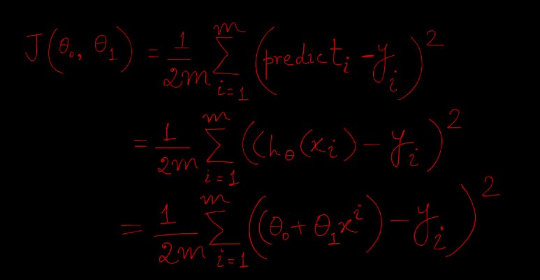
Now the famous Mean Squared Error function which measure the difference between the actual dataset and the estimated value (the prediction)
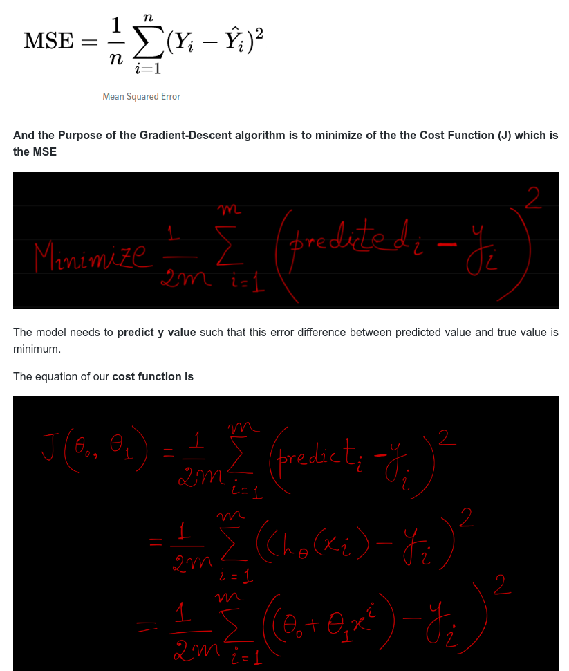
Now what exactly is the symbol Theta(θ) in the Cost funtion J(θ) ?
The θ theta values are the parameters or weights or coefficients as they are variously called. Lets see how.
The hypothesis equation is usually presented as
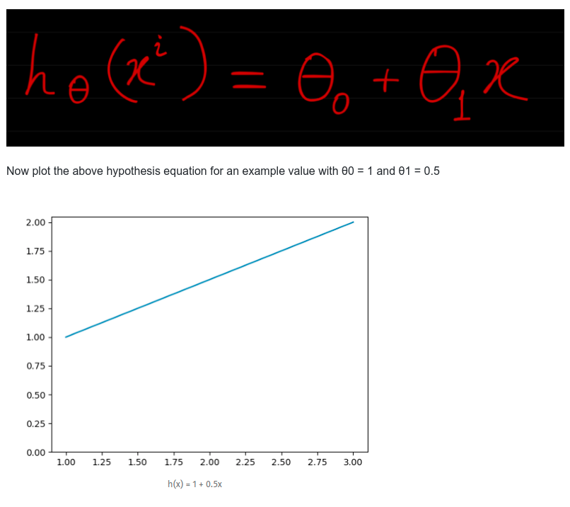
The goal of creating a model is to choose parameters, the θ values, so that h(x) is close to y for the training data, x and y.
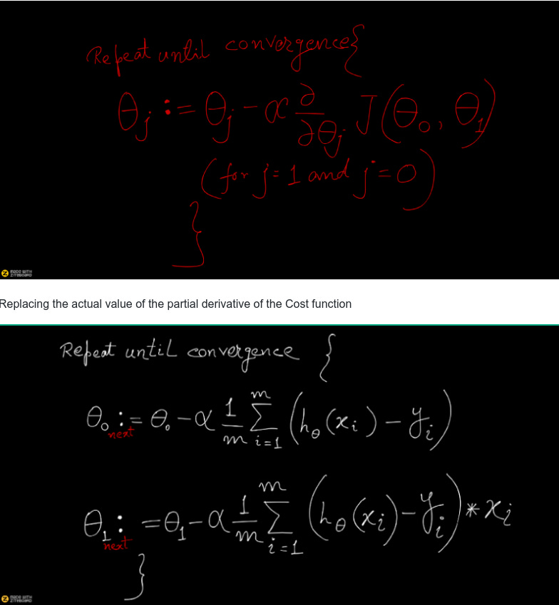
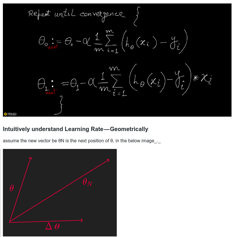
Now the key steps of the Gradient Descent process can be summarized as below.
Given m number of data set items in our learning set, with x and y values, we must find the best fit line represented by the hypothesis equation
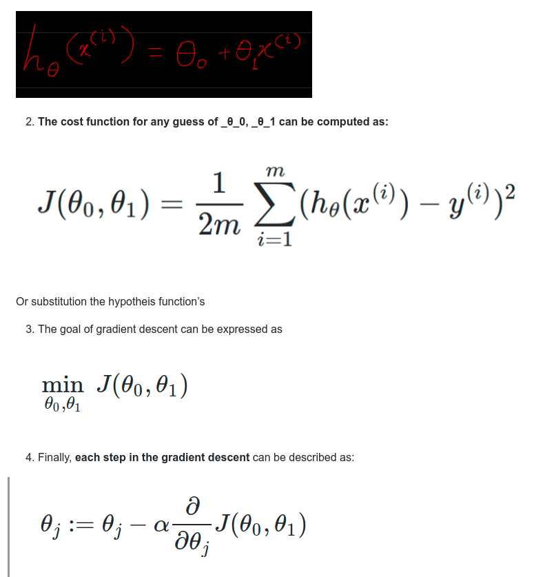
for j=0 and j=1 with α representing rate of learning or rate of step and is a constant.
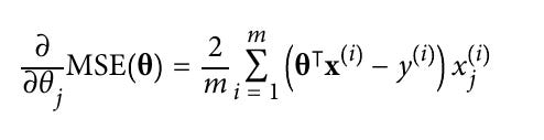
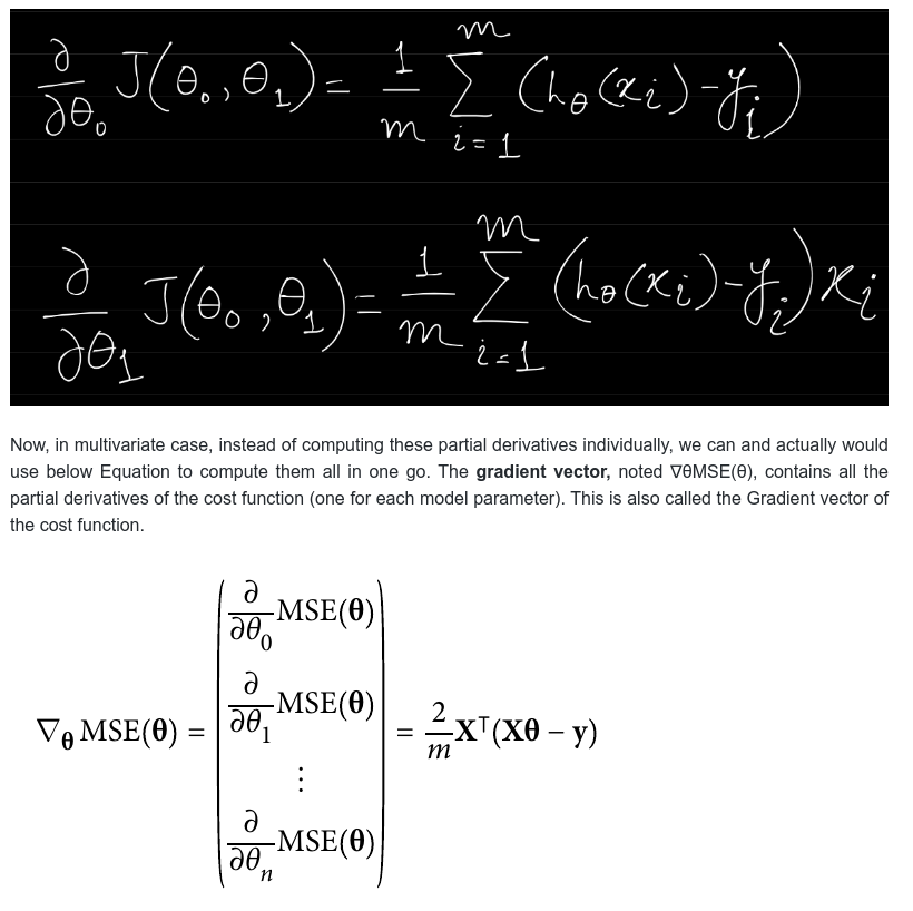
Now we know the equation after taking the partial derivative of the cost function (which I will derive below ) is the following
Explanataions of the notations
m is the number of instances in the dataset you are measuring the MSE on
x(i) is a vector of all the feature values (excluding the label) of the ith instance in the dataset, and y(i) is its label (the desired output value for that instance).
h is your system’s prediction function, also called a hypothesis. When your system is given an instance’s feature vector x(i), it outputs a predicted value ŷ(i) = h(x(i)) for that instance (ŷ is pronounced “y-hat”).
But now, to implement Gradient Descent, we need to compute the gradient of the cost function with regard to each model parameter θj. In other words, we need to calculate how much the cost function will change if we change θj just a little bit. This is called a partial derivative. It is like asking “What is the slope of the mountain under my feet if I face east?” and then asking the same question facing north (and so on for all other dimensions or directions ).
And the Partial derivatives of the cost function(Mean Squared Error) is as below in general mathematical form
And below are the actual derivation of the paritial derivative of the MSE.
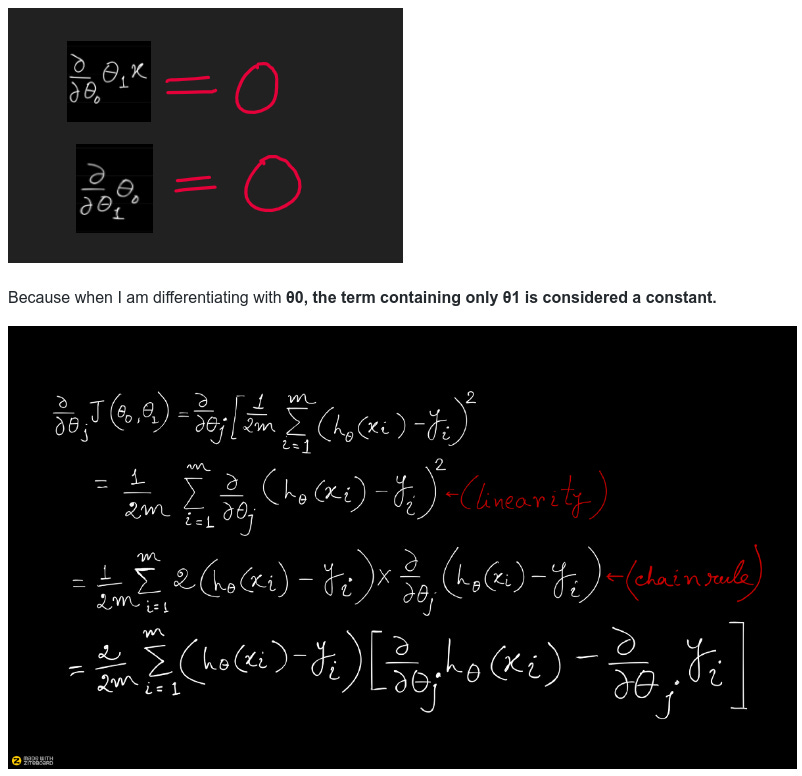
And now we will see many of the Calculus topics we discussed above will be used in the below derivation. Specifically, technique of the partial derivative and the chain rule is being applied in the below. So I am doing here is taking the cost function and then taking a partial derivative with respect to θ0 and θ1
First recount the following properties of Differential Calculus
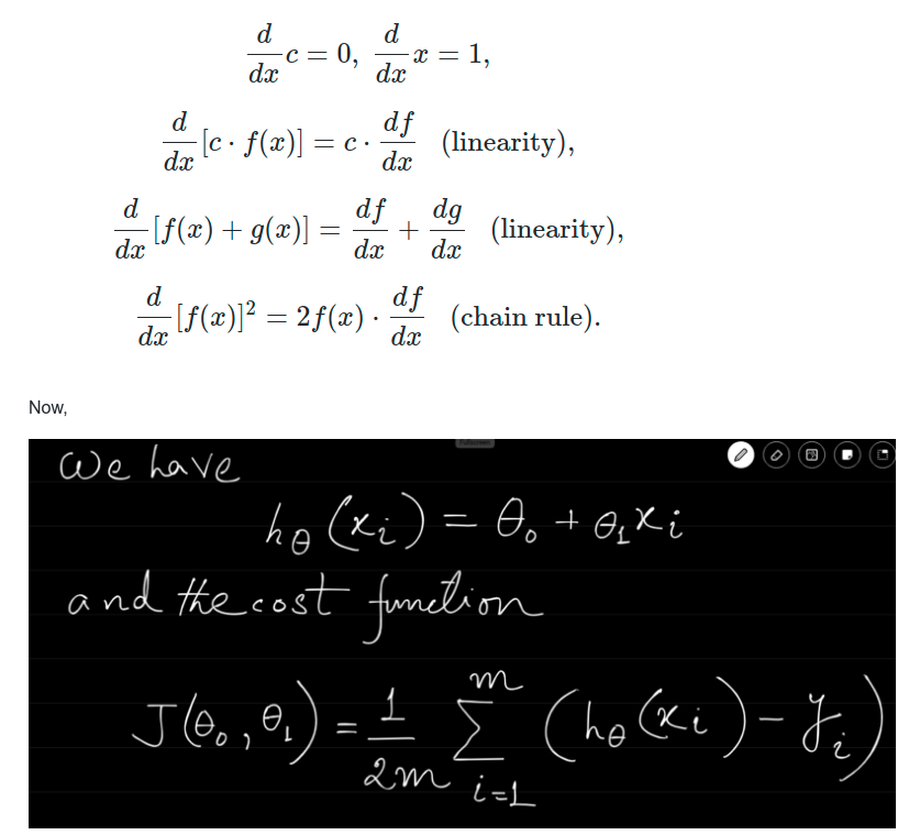
We first compute the individual partial derivative w.r.t. θ0 and θ1.
Now, partial differentiation is used in multivariable calculus, where functions are expressed in terms of at least 2 variables (i.e. the function depends on at least 2 variables). That's the reason here, that we need to get the partial derivative because from above we can see that the Cost function J is a function of 2 variables θ0 and θ1
For the below derivation, recount the rule of Partial Derivative, when I have a function f(x,y) of two variables (x and y) — to find its partial derivative with respect to x we treat y as a constant. Similarly to find the partial derivative with respect to y, we treat x as a constant.
And in below h(x) function is a function of two variables θ0 and θ1
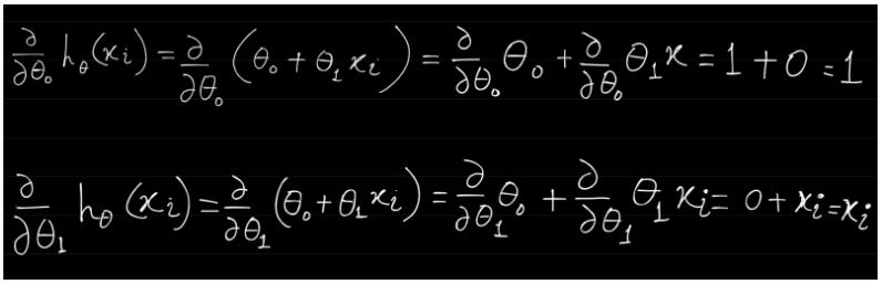
The above individual values will be required below (you will soon see). Now we want to compute the partial derivatives of the cost function J(_θ_0,_θ_1).
Special Note on Partial Derivative in the above equations — in the first equation (for finding derivative wrt θ0) the derivatives of the second term is zero because it does not contain the variable θ0, so the second term is treated as a constant term.
E.g. Calculate ∂f/∂x∂f/∂x for the following function_
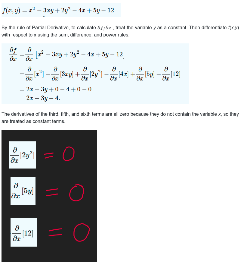
Similarly, in our Cost function,
Continue simplifying the last expression above further
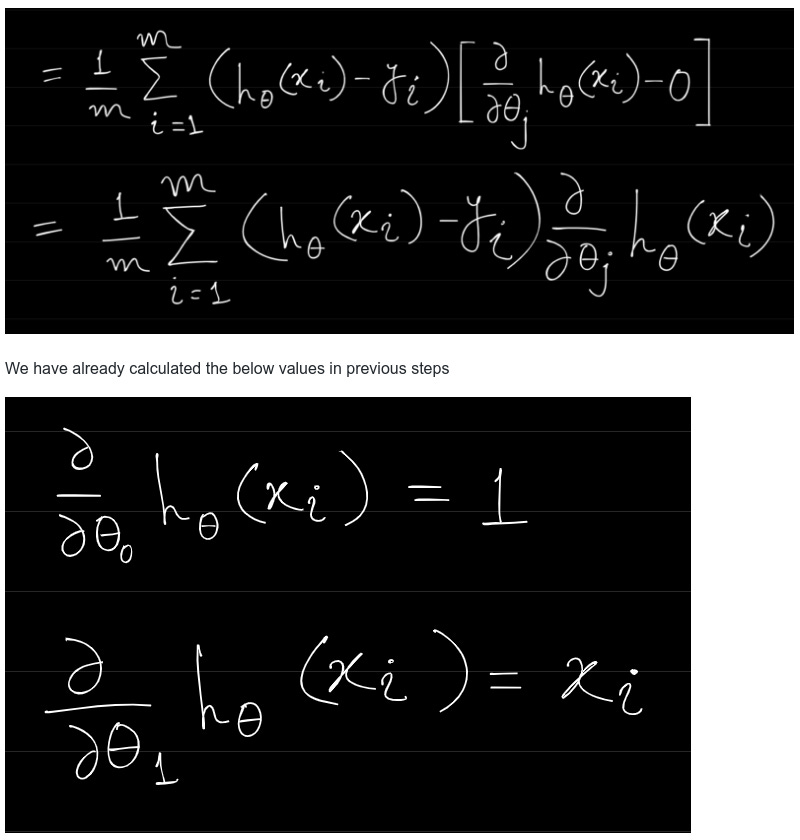
Now finally, we substitute the above values in the second portion of partial derivative of Cost function we get the final partial derivative result of Cost function in the below form.
Notice that this formula involves calculations over the full training set X, at each Gradient Descent step! This is why the algorithm is called Batch Gradient Descent: it uses the whole batch or the full set of training data at every step. As a result it is terribly slow on very large training sets. Thats why for big data set we have much faster Gradient Descent algorithms (Stochastic Gradient Descent).
And once the Gradient Descent process starts, as we discussed above the rules of Increasing and Decreasing function to minimalize cost function — Once you have the gradient vector, which points uphill, just go in the opposite direc‐ tion to go downhill. This means subtracting ∇θMSE(θ) from θ. This is where the learning rate alpha comes into play - multiply the gradient vector by η to determine the size of the downhill step.
Gradient Descent step / Learning Rate
Each iteration the coefficients, called weights (w) in machine learning language are updated using the equation:
The above is a general form for both θ0 and θ1, and below I am breaking down that further with the exact formulae for θ0 and θ1 and also substitution the actual result of the partial derivative of the cost function.
In above image, the new vector θN, has been calculated with by the rule of ‘Parallelogram Law of Vector Addition’
If two vectors acting simultaneously at a point can be represented both in magnitude and direction by the adjacent sides of a parallelogram drawn from a point, then the resultant vector is represented both in magnitude and direction by the diagonal of the parallelogram passing through that point.
Vector θ is moving in the direction of the vector Δθ . And the above image is without any learning rate, where θN moves all the way fully decided by the vector Δθ. But we don't want that to happen, as large movement of θ will give rise to a situation where we will mss the absolute minimum of the loss function.
So we adjust this large changes by a scaler alpha (α ) or learning rate, which is generally less than 1 usually 0.01 or 0.02 etc. So the movement of θN in the direction of Δθ will be scaled down by this factor alpha (α ).
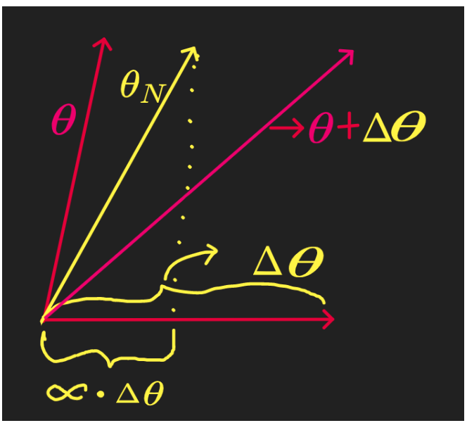
And that's the significance of Learning Rate.
Intuitive Understanding of the movement of the Theta (θ ) at each step during Gradient Descent
First take a Increasing function, the right portion of the below graph.
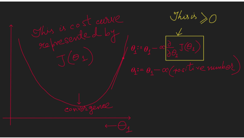
In the above to calculate the next value of Coefficient Theta (θ ) we are deducting a positive number from the current value of Theta (θ ). Hence in this case to find the convergence (the minimum point of the Cost function) Theta (θ ) needs to move towards left with each iteration.
Now take a Decreasing function, the left portion of the below graph.
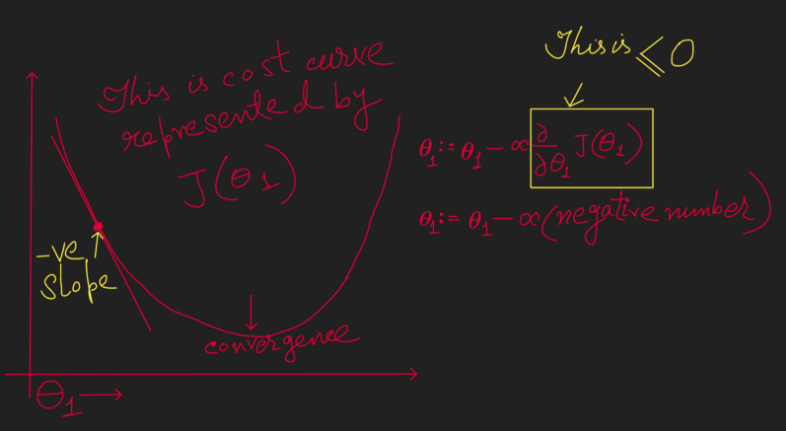
In the above to calculate the next value of Coefficient Theta (θ ) we are deducting a negative number from the current value of Theta (θ ). Hence in this case to find the convergence (the minimum point of the Cost function) Theta (θ ) needs to move towards right with each iteration.
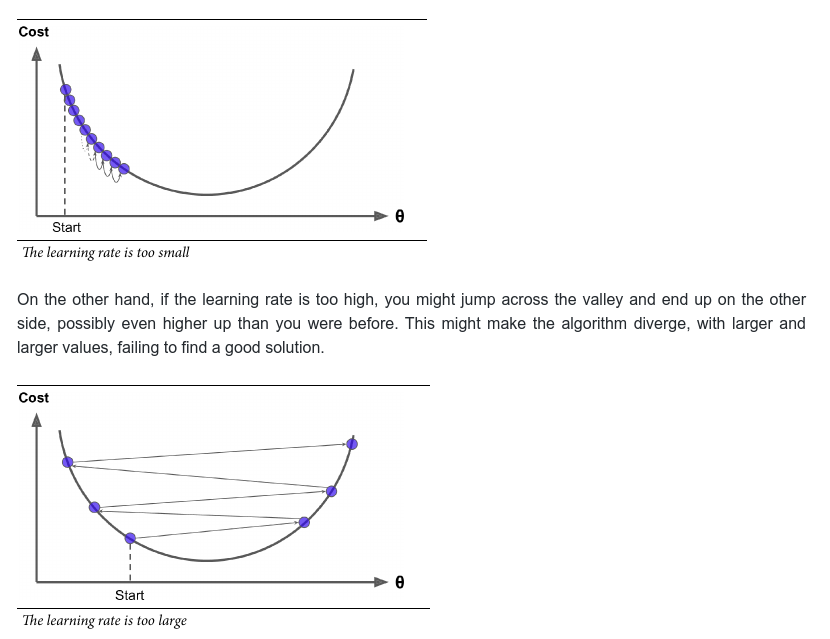
The learning step size is proportional to the slope of the cost function, so the steps gradually get smaller as the parameters approach the minimum. An important parameter in Gradient Descent is the size of the steps, determined by the learning rate hyperparameter. If the learning rate is too small, then the algorithm will have to go through many iterations to converge, which will take a long time
The most commonly used Learning Rates are: 0.001, 0.003, 0.01, 0.03, 0.1, 0.3.
Bonus Point-1: Multivariate Linear Regression — some notes
Multiple linear regression is an extension of bivariate linear regression, in which we have one dependent variable and two or more independent variables. In multiple linear regression analysis the regression model for p number of variables and n number of observations can be describe with below set of equations.
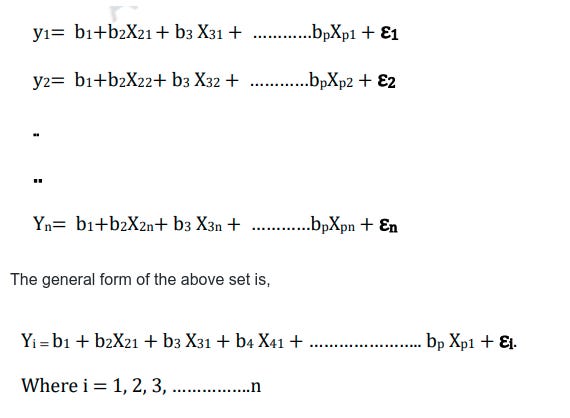
Each line in the above set of equations represents the entries of p variable for one observation, if there are n observations, there will be n such lines i.e. n number of equations. This general form can generate all n above equations by putting values for i from 1 to n.
The matrix form of the above set of equations will be
Where Y, B and ε are column vectors of px1 dimensions and X is the main data matrix of nxp dimensions i.e. n rows and p columns. (here convention of writing row number first and column number next has been interchanged to suit to the equation formation). In a multiple linear regression analysis also the problem is to find out the regression coefficients b1, b2, b3, ……bp. of the optimal line i.e. the least square line.
Now, as we recount that the the general form of the hypothesis equation in case of univariate linear regression was as below
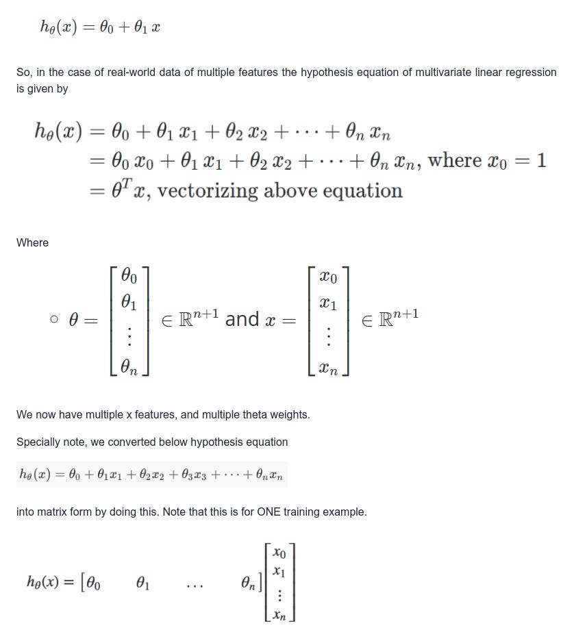
We now have multiple x features, and multiple theta weights.
Specially note, we converted below hypothesis equation
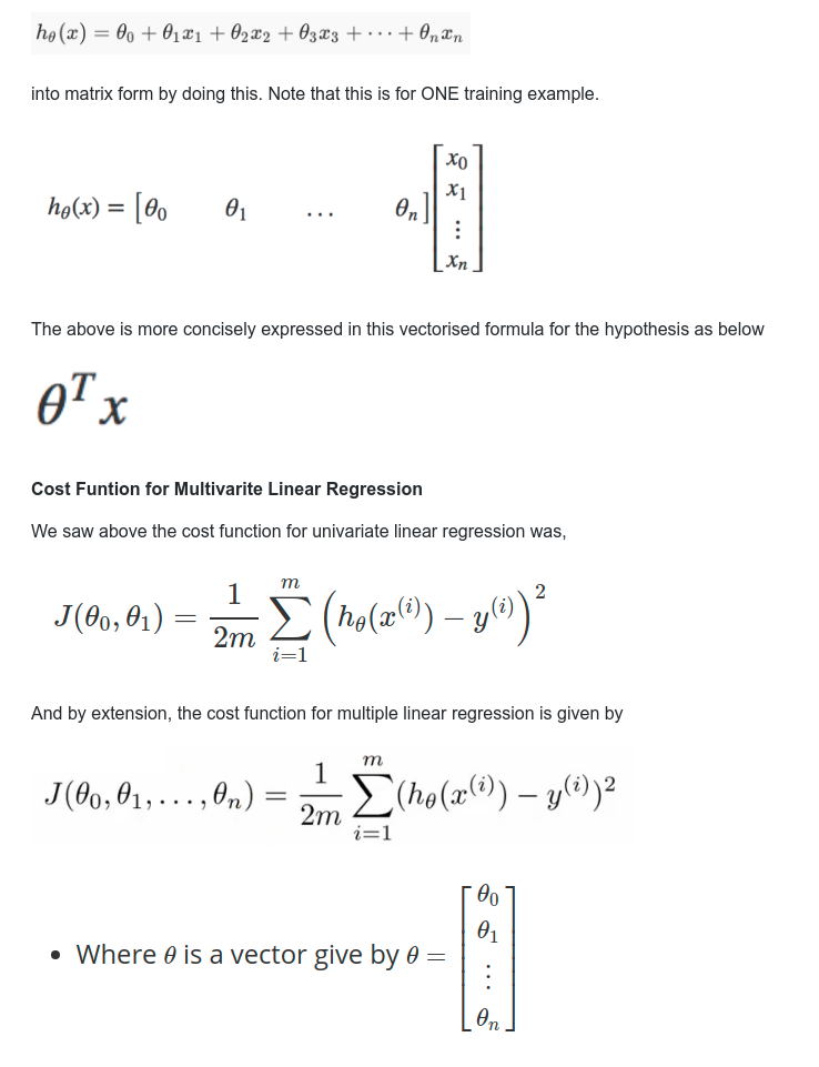
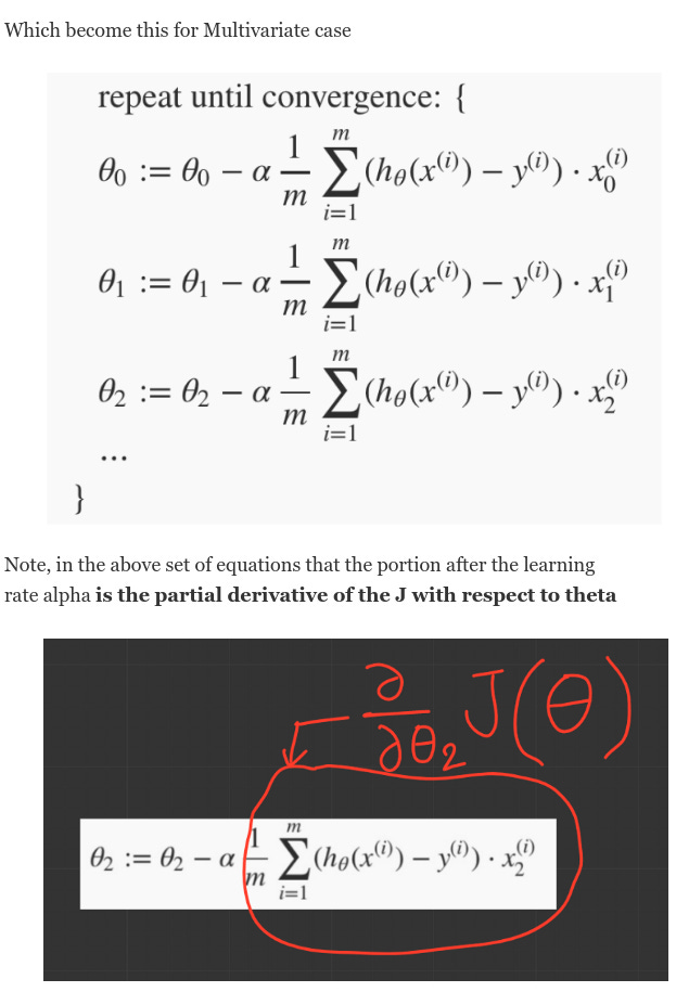
Gradient Descent for Multivariate Linear Regression
Which become this for Multivariate case
Bonus Point-2: — Ordinary Least Square (OLS) method
If instead of Gradient Descent we wanted to come up with a model to fit the data with a competing technique called Ordinary Least Square then that steps would go something like this.
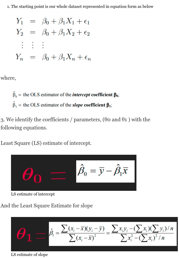
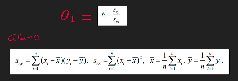
Theta_1Theta1 could also be expressed as below which is just a little bit more implications of the above.
Mathematical derivation of the above equations
Recount that the starting point for deriving the formulas for the OLS intercept and slope coefficient. That problem was below
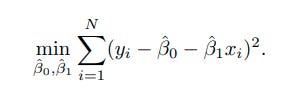
And we know that in calculus, a univariate optimization involves taking the derivative and setting equal to 0. So, this minimization problem above is solved by setting the partial derivatives equal to 0. That is, take the derivative of the above equation with respect to β 0 and set it equal to 0. We then do the same thing for β 1. This gives us,
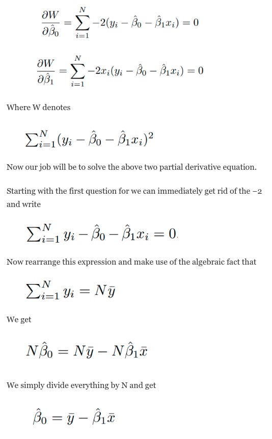
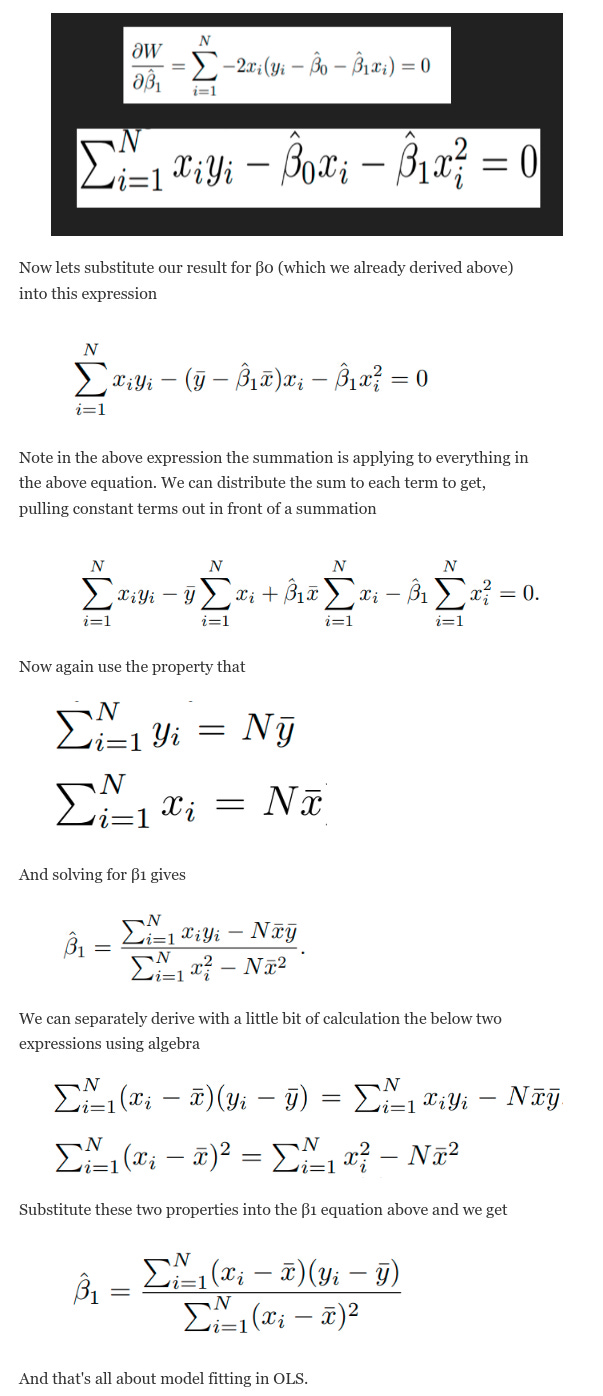
Similarly, now consider the second equation above. We first get rid of the −2 and rearrange the Equation to get
Thanks for reading :) :)