
DCGAN from Scratch with Tensorflow Keras
Create Fake Images from CELEB-A Dataset

Link to my Kaggle Notebook with full codes.
What is Facial Attribute Prediction?
Facial Attribute prediction is a Computer Vision (CV) task about deducing the set of attributes belonging to a face. Example attributes are the color of hair, hairstyle, age, gender, etc.
Facial attribute analysis has received considerable attention when deep learning techniques made remarkable breakthroughs in this field over the past few years.
Deep learning based facial attribute analysis consists of two basic sub-issues:
facial attribute estimation (FAE), which recognizes whether facial attributes are present in given images, and
facial attribute manipulation (FAM), which synthesizes or removes desired facial attributes.
Getting to know the CELEB-A Dataset
202,599 number of face images of various celebrities 10,177 unique identities, but names of identities are not given 40 binary attribute annotations per image 5 landmark locations
Data Files
img_align_celeba.zip: All the face images, cropped and aligned
list_eval_partition.csv: Recommended partitioning of images into training, validation, testing sets. Images 1–162770 are training, 162771–182637 are validation, 182638–202599 are testing
list_bbox_celeba.csv: Bounding box information for each image. “x_1” and “y_1” represent the upper left point coordinate of bounding box. “width” and “height” represent the width and height of bounding box
list_landmarks_align_celeba.csv: Image landmarks and their respective coordinates. There are 5 landmarks: left eye, right eye, nose, left mouth, right mouth
list_attr_celeba.csv: Attribute labels for each image. There are 40 attributes. “1” represents positive while “-1” represents negative
Fundamental way GAN Works
GAN contains two networks which has two competing objectives:
Generator: the generator generates new data instances that are “similar” to the training data, in our case celebA images. Generator takes random latent vector and outputs a “fake” image of the same size as our reshaped celebA image.
Discriminator: the discriminator evaluate the authenticity of provided images; it classifies the images from the generator and the original image. Discriminator takes true of fake images and outputs the probability estimate ranging between 0 and 1.
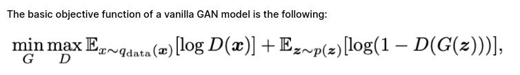
Here, D refers to the discriminator network, while G obviously refers to the generator.
As the formula shows, the generator optimizes for maximally confusing the discriminator, by trying to make it output high probabilities for fake data samples.
On the contrary, the discriminator tries to become better at distinguishing samples coming from G from samples coming from the real distribution.
The GAN training process consists of a two-player minimax game in which D is adapted to minimize the discrimination error between real and generated samples, and G is adapted to maximize the probability of D making a mistake. When G does a good enough job to fool D, the output probability should be close to 1.
Regular Neural Network vs CNN
Unlike a regular feed-forward neural network whose neurons are arranged in flat, fully connected layers, layers in a ConvNet are arranged in three dimensions (width × height × depth).
Convolutions are performed by sliding one or more filters (the smaller Matrix which is the Kernel of the Current Layer) over the input layer. Each filter has a relatively small receptive field (width × height) but always extends through the entire depth of the input volume.
At every step as it slides across the input, each filter outputs a single activation value: the dot product between the input values and the filter entries.
Convolutional Neural Networks (CNNs) are neural networks with architectural constraints to reduce computational complexity and ensure translational invariance (the network interprets input patterns the same regardless of translation — in terms of image recognition: a banana is a banana regardless of where it is in the image).
Convolutional Neural Networks have three important architectural features.
Local Connectivity: Neurons in one layer are only connected to neurons in the next layer that is spatially close to them. This design trims the vast majority of connections between consecutive layers but keeps the ones that carry the most useful information. The assumption made here is that the input data has spatial significance, or in the example of computer vision, the relationship between two distant pixels is probably less significant than two close neighbors.
Shared Weights: This is the concept that makes CNNs “convolutional.” By forcing the neurons of one layer to share weights, the forward pass (feeding data through the network) becomes the equivalent of convolving a filter over the image to produce a new image. The training of CNNs then becomes the task of learning filters (deciding what features you should look for in the data.)
Pooling and ReLU: CNNs have two non-linearities: pooling layers and ReLU functions. Pooling layers consider a block of input data and simply pass on the maximum value. Doing this reduces the size of the output and requires no added parameters to learn, so pooling layers are often used to regulate the size of the network and keep the system below a computational limit. The ReLU function takes one input, x, and returns the maximum of {0, x}. ReLU(x) = argmax(x, 0). This introduces a similar effect to tanh(x) or sigmoid(x) as non-linearities to increase the model’s expressive power.
Deep Convolutional GANs (DCGANs)
Deep Convolutional GANs (DCGANs) introduced convolutions to the generator and discriminator networks.
However, this was not simply a matter of adding convolutional layers to the model, since training became even more unstable.
Generator Architecture

The generator network of a DCGAN contains 4 hidden layers (we treat the input layer as the 1st hidden layer for simplicity) and 1 output layer. Transposed convolution layers are used in hidden layers, which are followed by batch normalization layers and ReLU activation functions. The output layer is also a transposed convolution layer and Tanh is used as the activation function.
The 2nd, 3rd, and 4th hidden layers and the output layer have a stride value of 2. The 1st layer has a padding value of 0 and the other layers have a padding value of 1. As the image (feature map) sizes increase by two in deeper layers, the numbers of channels are decreasing by half. This is a common convention in the architecture design of neural networks. All kernel sizes of transposed convolution layers are set to 4 x 4. The output channel can be either 1 or 3, depending on whether you want to generate grayscale images or color images.
The architecture of a discriminator
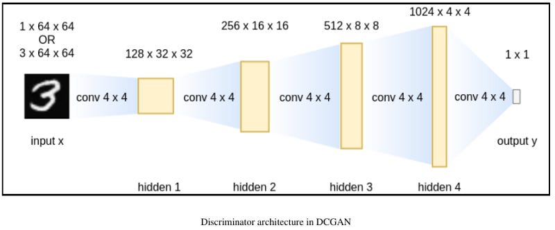
The discriminator network of a DCGAN consists of 4 hidden layers (again, we treat the input layer as the 1st hidden layer) and 1 output layer. Convolution layers are used in all layers, which are followed by batch normalization layers except that the first layer does not have batch normalization. LeakyReLU activation functions are used in the hidden layers and Sigmoid is used for the output layer. The architecture of the discriminator is shown in the following:
The input channel can be either 1 or 3, depending on whether you are dealing with grayscale images or color images. All hidden layers have a stride value of 2 and a padding value of 1 so that their output image sizes will be half the input images. As image sizes increase in deeper layers, the numbers of channels are increasing by twice. All kernels in convolution layers are of a size of 4 x 4. The output layer has a stride value of 1 and a padding value of 0. It maps 4 x 4 feature maps to single values so that the Sigmoid function can transform the value into prediction confidence.
Several tricks had to be applied to make DCGANs stable and useful:
Batch normalization was applied to both the generator and the discriminator network Dropout is used as a regularization technique The generator needed a way to upsample the random input vector to an output image. Transposing convolutional layers is employed here LeakyRelu and TanH activations are used throughout both networks
How Reverse ConvNets works in DCGAN
ConvNets have traditionally been used for image classification tasks, in which the network takes in an image with the dimensions height × width × number of color channels as input and — through a series of convolutional layers — outputs a single vector of class scores, with the dimensions 1 × n, where n is the number of class labels.
In DCGAN, under the Generator part, to generate an image by using the ConvNet architecture, we reverse the process: instead of taking an image and processing it into a vector, we take a vector and up-size it to an image.
So, overall, the core to the DCGAN architecture uses a standard CNN architecture on the discriminative model.
But for the generator, convolutions are replaced with up-convolutions, so the representation at each layer of the generator is actually successively larger, as it maps from a low-dimensional latent vector onto a high-dimensional image.
Let's start coding and preparing the CELEB-A Dataset
Transposed Convolutions
Lets first take a look at normal convolutions

The 2×2 kernel produces a 2×2 output when convolving over a 3×3 image.
But I want to work in the opposite direction, i.e., to use a smaller input and to learn its larger representation, being the following:

That's where the Transposed convolutions in the Keras API come to help.
The Conv2DTranspose layer learns a number of filters, similar to the regular Conv2D layer.
Remember that the transpose layer simply swaps the backward and forward pass, keeping the rest of the operations the same!
As the transposed convolution will also slide over the input, we must specify a kernel_size, as with the normal convolution. Similarly, we got to specify strides, output_padding
UpSampling2D vs Conv2DTranspose in Keras
UpSampling2D is just a simple scaling up of the image by using a nearest neighbor or bilinear upsampling, so nothing smart. The advantage is it’s cheap.
Conv2DTranspose is a convolution operation whose kernel is learnt (just like normal conv2d operation) while training your model. Using Conv2DTranspose will also upsample its input but the key difference is the model should learn what is the best upsampling for the job.
Generator
I use Leaky relu activations in the hidden layer neurons, and sigmoids for the output layers. Originally, ReLU was recommend for use in the generator model and LeakyReLU was recommended for use in the discriminator model, although more recently, the LeakyReLU is recommended in both models.
The generator consists of convolutional-transpose layers, batch normalization layers, and ReLU activations. The output will be a 3x64x64 RGB image.
Use of Batch Normalization
Batch normalization standardizes the activations from a prior layer to have a zero mean and unit variance. This has the effect of stabilizing the training process.
Batch normalization limits the amount by which updating the parameters in the previous layers can affect the distribution of inputs received by the current layer. This decreases any unwanted interdependence between parameters across layers, which helps speed up the network training process and increase its robustness, especially when it comes to network parameter initialization.
Batch normalization is used after the activation of convolution in the discriminator model and after transpose convolutional layers in the generator model.
It is added to the model after the hidden layer, but before the activation, such as LeakyReLU.
Now the code for Generator and Discriminator
DCGAN — Combining Generator and Discriminator
The combined model is stacked generator and discriminator
Setting discriminator.trainable to False.
Why would we want to do this?
Well, we aren’t going to be training the generator model directly — we are going to be combining the generator and discriminator into a single model, then training that. This allows the generator to understand the discriminator so it can update itself more effectively.
Setting discriminator.trainable to False will only affect the copy of the discriminator in the combined model. This is good! If the copy of the discriminator in the combined model were trainable, it would update itself to be worse at classifying images.
To combine the generator and discriminator, we will be calling the discriminator on the output of the generator.
GAN =Sequential([generator,discriminator])
discriminator.compile(optimizer='adam',loss='binary_crossentropy')
When we train this network, we don't want to train the discriminator network,_
so make it non-trainable before we add it to the adversarial model._
discriminator.trainable = False
GAN.compile(optimizer='adam',loss='binary_crossentropy')
GAN.layers
GAN.summary()
Final DCGAN Training
Training GANs is an art form itself, as incorrect hyperparameter settings lead to mode collapse. So play with different hyperparameters to obtain better results.
Final Training Architecture of a DCGAN
Initially, both of the networks are naive and have random weights.
The standard process to train a DCGAN network is to first train the discriminator on the batch of samples.
To do this, we need fake samples as well as real samples. We already have the real samples, so we now need to generate the fake samples.
To generate fake samples, create a latent vector of a shape of (100,) over a uniform distribution. Feed this latent vector to the untrained generator network. The generator network will generate fake samples that we use to train our discriminator network. So the training loop begins with the generator receiving a random seed as input. That seed is used to produce an image.
Concatenate the real images and the fake images to create a new set of sample images. We also need to create an array of labels: label 1 for real images and label 0 for fake images.
The discriminator is then used to classify real images (drawn from the training set) and fakes images (produced by the generator).
The loss is calculated for each of these models In the process defined below I am training the generator and discriminator simultaneously.
DCGAN is super sensitive
Here, even when we only train a GAN to manipulate 1D data, we have to use multiple techniques to ensure stable training. A lot of things could go wrong in the training of GANs. For example, either a generator or a discriminator could overfit if one or the other does not converge. Sometimes, the generator only generates a handful of sample varieties. This is called mode collapse.
It’s important that the generator and discriminator do not overpower each other (e.g., that they train at a similar rate).
At the beginning of the training, the generated images will look like random noise. As training progresses, the generated images will look increasingly real just like original celeb-a images. After about 300 epochs, they resemble almost the original.
Since we are training two models at once, the discriminator and the generator, we can’t rely on Keras’ .fit function. Instead, we have to manually loop through each epoch and fit the models on batches.
That wraps up the training and you can now see examples of the fake images generated after the above training with the below plotting code.

Of course, the above images are not yet perfect, as I did not use the full 200k training data.
Link to my Kaggle Notebook with full codes.