🧠 DeepSeek just improved the Transformer architecture
DeepSeek optimizes core Transformer design, AI DRAM demand triggers supercycle, and The Information lays out sharp 2026 LLM predictions.
Read time: 12 min
📚 Browse past editions here.
( I publish this newletter daily. Noise-free, actionable, applied-AI developments only).
⚡In today’s Edition (2-Jan-2026):
🧠 DeepSeek dropped a core Transformer architecture improvement.
🏆 The Information’s AI predictions for 2026
📡A dynamic random-access memory (DRAM) “supercycle” has started in Q3 2025 and could run to Q4 2027, as AI datacenters pull supply away from consumer PCs and push prices up.
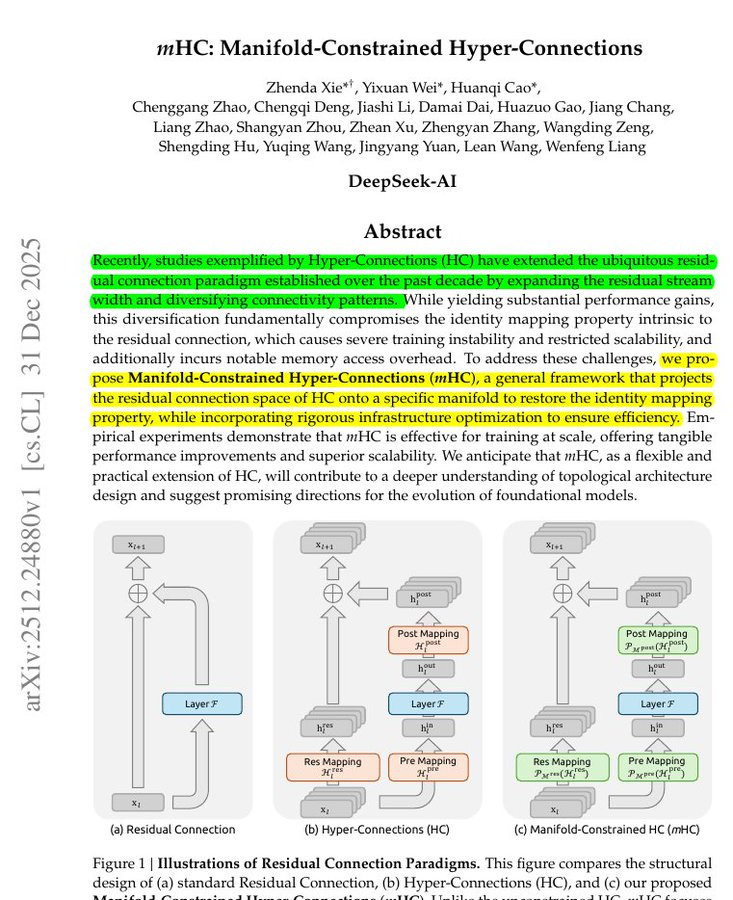
🚨 BREAKING: DeepSeek dropped a core Transformer architecture improvement.
Each block in this original transformer architecture does some work (self attention or a small feed forward network), then it adds the block’s input back onto the block’s output, which is why people describe it as a “main path” plus a “shortcut path.” Hyper-Connections is a drop-in change to that shortcut path, because instead of carrying 1 stream of activations through the stack, the model carries a small bundle of parallel streams, then it learns how to mix them before a block and after a block.
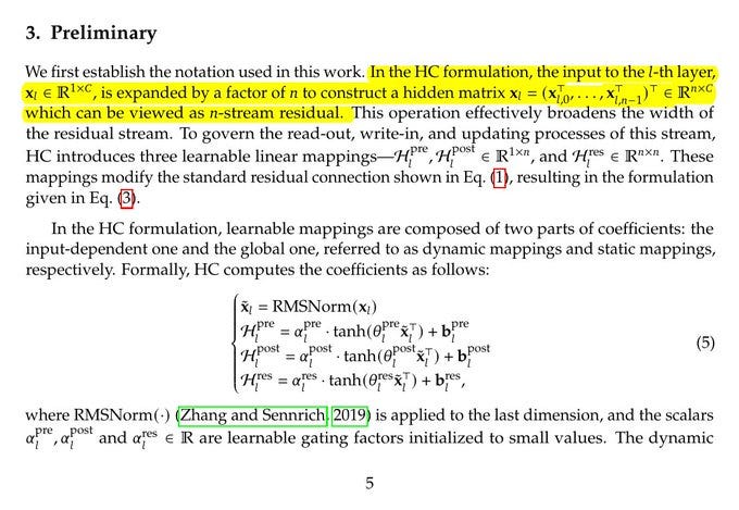
Standard Transformers pass information through 1 residual stream. Hyper-Connections turn that into n parallel streams, like n lanes on a highway. Small learned matrices decide how much of each lane should mix into the others at every layer.
In a normal residual connection, each layer takes the current hidden state, runs a transformation, then adds the original back, so information can flow forward without getting stuck. In this new Hyper-Connections, the layer does not see just 1 hidden state, it sees a small bundle of them, and before the layer it learns how to mix that bundle into the input it will process.
So in a traditional transformer block, wherever you normally do “output equals input plus block(input),” Hyper-Connections turns that into “output bundle equals a learned mix of the input bundle plus the block applied to a learned mix,” so the shortcut becomes more flexible than a plain add. After this learned layer, the “Hyper-Connections” mechanism again learns how to mix the transformed result back into the bundle, so different lanes can carry different kinds of information, and the model can route signal through the shortcut in a more flexible way.
The catch is that if those learned mixing weights are unconstrained, stacking many blocks can make signals gradually blow up or fade out, and training becomes unstable in big models. This paper proposes mHC, which keeps Hyper-Connections but forces every mixing step to behave like a safe averaging operation, so the shortcut stays stable while the transformer still gets the extra flexibility from multiple lanes.
---
The paper shows this stays stable at 27B scale and beats both a baseline and unconstrained Hyper-Connections on common benchmarks. HC can hit about 3000x residual amplification, mHC keeps it around 1.6x.
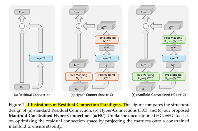
This image compares 3 ways to build the shortcut path that carries information around a layer in a transformer.
The left panel is the normal residual connection, where the model adds the layer output back to the original input so training stays steady as depth grows. The middle panel is Hyper-Connections, where the model keeps several parallel shortcut streams and learns how to mix them before the layer, around the layer, and after the layer, which can help quality but can also make the shortcut accidentally amplify or shrink signals when many layers stack. The right panel is mHC, which keeps the same Hyper-Connections idea but forces those mixing steps to stay in a constrained safe shape every time, so the shortcut behaves like a controlled blend and stays stable at large scale.
What “hyper-connection” means here.
You widen the residual from size C to n×C, treat it as n streams, and learn 3 tiny mixing pieces per layer. One mixes the residual streams with each other, this is the crucial one. One gathers from the streams into the layer. One writes results back to the streams. The paper’s contribution is to keep the first one in the safe “doubly stochastic” set, so it mixes without amplifying.
🧯 The mHC constraint, mixing without blowing up
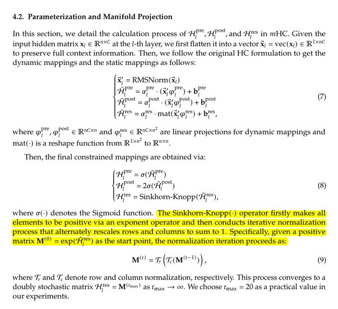
mHC keeps the multi-stream setup, but forces the stream-mixing table to live inside a safe set of non-negative weights. Every row and every column is forced to add up to 1, so each output stream becomes a weighted average of the input streams.
A weighted average cannot scale the overall magnitude beyond 1x, so forward activations and backward gradients stop exploding. Stacking many layers stays safe because multiplying 2 of these tables still preserves the same row-and-column-sum rule.
The paper describes the geometry as Birkhoff polytope, which can be thought of as mixtures of pure permutations that shuffle streams without scaling them. mHC also keeps the read-in and write-back weights non-negative, which reduces signal cancellation from positive and negative coefficients fighting each other.
🚧 Why HC can get slow, even if FLOPs look fine
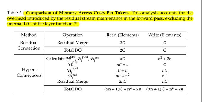
Making the residual stream n times wider also makes it n times heavier to move through GPU memory, which hurts when training is memory-bandwidth limited. The paper points at the “memory wall” problem, where reading and writing activations dominates runtime even if raw compute stays similar.
A standard residual merge mainly reads the current state and the block output, then writes 1 merged result, but HC adds extra reads and writes for the pre-map, post-map, and stream-mix steps. Table 2 shows this I/O overhead grows roughly with n, which is why naive HC can lose a lot of throughput when n is 4 without fused kernels.
Because these mapping weights depend on the input, intermediate activations must be kept for backpropagation, which pushes GPU memory use up and makes checkpointing more likely. Pipeline parallelism gets hit too, because pushing n streams across stage boundaries multiplies communication and creates bigger idle bubbles.
🛠️ The engineering that keeps mHC practical
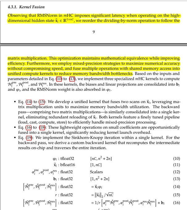
The paper treats GPU kernels as part of the architecture, because the constraint is useless if it turns into a slow pile of tiny kernel launches. It combines steps that touch the same memory into fused kernels, so the hidden state is loaded once, processed, and written back without extra trips.
The Root Mean Square Layer Normalization division is reordered to happen after the big matrix multiply, which keeps the math equivalent but reduces latency on the huge nC vector. Precision is mixed so accumulation happens in float32 while storage stays in bfloat16 where possible, and TileLang is used to implement most of the custom kernels.
The Sinkhorn-Knopp loop is packed into 1 kernel, and the backward pass recomputes needed intermediates on-chip instead of saving them. A recomputation scheme throws away intermediate activations in the forward pass and re-runs the lightweight mHC kernels during backprop, trading extra compute for lower peak memory.
Communication is overlapped with compute using an extended DualPipe schedule, including a high-priority stream for the Multi-Layer Perceptron, MLP, residual-merge kernel so pipeline sends do not stall. With these system tricks, the paper reports only 6.7% extra training time when n is 4.
🧪 What the experiments actually show
The experiments pretrain Mixture-of-Experts, MoE, language models based on the DeepSeek-V3 setup, comparing a baseline, HC, and mHC with n set to 4. The main run is a 27B model, with extra runs at 3B and 9B for compute scaling, plus a 3B run trained for about 1T tokens to study token scaling.
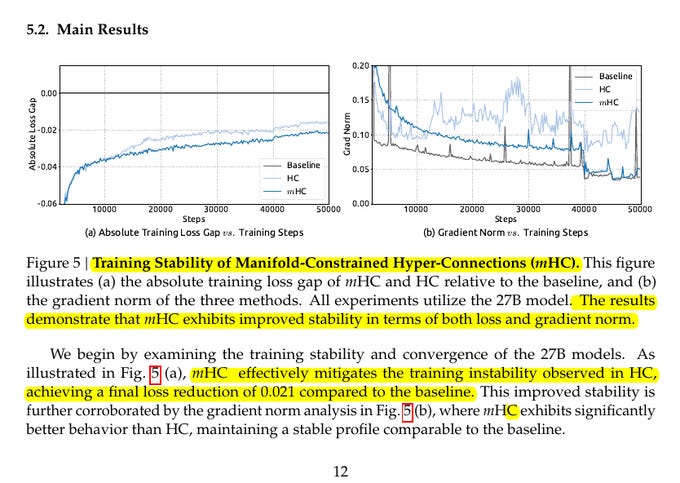
On the 27B run, mHC keeps training smooth where HC shows a loss spike and a matching jump in gradient norm. After training finishes, the paper reports the mHC run lands 0.021 lower in loss than the baseline.
On downstream benchmarks, mHC beats the baseline on all 8 tasks in Table 4, for example 51.0 on BBH versus 43.8, and 53.9 on DROP versus 47.0. Compared with HC, mHC is usually better too, including 57.6 versus 56.3 on TriviaQA, and an extra 2.1% on BBH plus 2.3% on DROP. The scaling plots show the advantage does not disappear as compute grows from 3B to 27B, and the within-run token curve stays ahead through training.
📉 Why the scary training spikes disappear with mHC
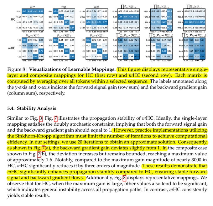
To explain why HC can blow up, the paper measures worst-case amplification through the stream-mixing stack, separately for the forward signal and the backward gradient. The forward metric tracks the largest absolute row-sum of the composite mixing map, and the backward metric tracks the largest absolute column-sum, so spikes are obvious.
In HC, the composite map can hit peaks around 3000, which matches exploding gradients and the mid-run loss surge seen in training. In mHC, the same measurement stays close to 1, and the reported composite peak is about 1.6, mostly because the Sinkhorn-Knopp projection is approximate at 20 iterations.
That is a stability jump of about 3 orders of magnitude, while still keeping the cross-stream mixing that made HC attractive. The matrix visualizations back this up, with HC showing large, messy values across many paths, while mHC stays non-negative and looks like controlled mixing.
So what does all this means for model training now.
The big win now is that you can try widening the residual stream with Hyper-Connections without betting the whole run on shaky optimization, because mHC is explicitly built to restore the identity-style stability that plain HC breaks.
That matters most in long, expensive pretrains where a single signal blow-up can waste a lot of compute, since the paper says HC can create unbounded amplification or attenuation across depth, which is exactly the kind of thing that shows up as loss spikes and nasty gradient norms.
Next great win is the memory traffic.
The plain traditional Hyper-Connections can slow training a lot even if compute looks “cheap” on paper, because the job becomes bottlenecked by extra memory movement and bigger pipeline sends. “Memory traffic” here means how many bytes each layer has to read from GPU memory and write back, because GPUs can sit idle if they are waiting on those reads and writes, which is the “memory wall” problem the paper calls out.
With the traditional the n-stream Hyper-Connections methods, residual design increases per-token memory access roughly proportional to n, increases activation memory needed for backprop, and even multiplies pipeline-parallel communication costs. mHC brings benefits here mainly because they treat this as a systems problem too, meaning fused kernels cut extra reads and writes, recomputation trims activation storage, and scheduling hides some communication, which is why they report only 6.7% overhead at n=4 in their setup.
For inference, that widening the residual stream under traditional Hyper-Connections, is naturally scary for latency, because decoder serving is often limited by memory bandwidth rather than raw compute, and extra residual streams mean more bytes moved per generated token unless kernels are very tight.
BUT, mHC is only “usable” if the implementation work is done, because they lean on fused kernels, mixed precision, selective recomputation, and communication overlap, and they report only 6.7% extra training time at n=4 once those pieces are in place.
🏆 The Information’s AI predictions for 2026:
OpenAI ships an AI research intern by Sept 2026
A major lab introduces a $1,000-per-month agent.
Gemini closes the gap with ChatGPT on weekly users.
The rise of Continual Learning could send AI compute to 100% inference and basically 0% training.
Continual learning, is when a model keeps updating after deployment instead of staying frozen until the next big training run. The key nuance is that continual learning does not magically remove training. It mostly changes when and where training happens.
Here is what actually changes if continual learning gets really good. Instead of “train for months, deploy for months”, you get “deploy, collect signals, do many small updates constantly”.
That can reduce some giant scheduled retrains, but it also creates new compute needs: frequent fine-tuning steps, lots of evaluation to avoid the model drifting or forgetting, safety checks, and infrastructure to manage many model versions. Even if each update is smaller than a frontier retrain, you might run them far more often, across far more product surfaces, for personalization and domain adaptation.
So in my opinon, their prediction that training compute goes to 0% is the part that feels directionally wrong. Also, IMO, with a breakthrough in “continual learning”, Nvidia’s stock will get another boost.
Nvidia sells the picks and shovels for both training and inference. If anything, continual learning can increase inference-side complexity, because you are not just serving forward passes, you are also managing memory, state, and sometimes update steps. That tends to push you toward more capable hardware, not less.
📡A dynamic random-access memory (DRAM) “supercycle” has started in Q3 2025 and could run to Q4 2027, as AI datacenters pull supply away from consumer PCs and push prices up.
Demand for RAM rising much faster than factories and packaging lines can expand.
The driver is high-bandwidth memory (HBM), which stacks DRAM close to a graphics processing unit (GPU) so accelerators can move model weights with very high bandwidth. Making HBM uses up about 3x as much factory wafer output as making the same amount of DDR5, so if a memory maker shifts production toward HBM, there is less capacity left to pump out regular PC RAM.
HBM is harder to manufacture because it gets stacked and then connected with extra packaging steps, so a bigger share of units can fail quality tests, which further reduces how many finished chips come out per wafer. Because HBM is higher margin, suppliers prioritize HBM and server parts like DDR5 RDIMM (registered dual inline memory module) and MRDIMM/MCRDIMM, leaving fewer bits for consumer DDR4 and DDR5.
TrendForce reported AI could consume about 20% of global DRAM wafer capacity in 2026, so even small allocation shifts can bite the PC channel. Original equipment manufacturers (OEMs) then face a higher bill of materials (BoM), and respond by raising prices, lowering default RAM, or delaying launches.
Dell has flagged increases like $130-$230 for 32GB systems and $520-$765 for 128GB systems, plus added cost for 1TB solid state drive (SSD) options. This squeeze is happenning because bandwidth-first AI memory and capacity-first PC memory share upstream wafers and packaging, so the best-paying demand gets served first.
That’s a wrap for today, see you all tomorrow.

