
Gravitational Waves Detection - Kaggle Competition


In this part, I shall go through the introduction on Gravitational waves, fundamentals of digital signal processing which is required to model gravitational waves, and how Machine-Learning and Deep-Learning have become one of the most crucial tool now to handle this fascinating phenomenon that was first proposed by Einstein himself in his landmark paper in 1916.
In the June of 1916, Einstein presented to the Prussian Academy of Sciences his paper, in which he first proposed the existence of gravitational waves, published later under the title, “Approximate Integration of the Field Equations of Gravitation”.
What is this Kaggle Competition all about
In this competition, we are provided with a training set of time series data containing simulated gravitational wave measurements from a network of 3 gravitational wave interferometers (LIGO Hanford, LIGO Livingston, and Virgo). Each time series contains either detector noise or detector noise plus a simulated gravitational wave signal. The task is to identify when a signal is present in the data (target=1).
So we need to use the training data along with the target value to build our model and make predictions on the test IDs in form of probability that the target exists for that ID.
So basically data science helping here by building models to filter out these noises from data-streams (which includes both noise frequencies and Gravitational Waves frequencies) so we can single out frequencies for Gravitational-Waves. This is very well-explained by Professor Rana Adhikari of Caltech and a member of the LIGO team, who were the first to measure gravitational waves. See his interview here )
Description of the 72GB Data Provided in Kaggle
We are provided with a train and test set of time series data containing simulated gravitational wave measurements from a network of 3 gravitational wave interferometers:
LIGO Hanford
LIGO Livingston
Virgo
Each time series contains either detector noise or detector noise plus a simulated gravitational wave signal.
The task is to identify when a signal is present in the data (target=1).
Each .npy data file contains 3 time series (1 coming for each detector) and each spans 2 sec and is sampled at 2,048 Hz.
And we have a total of 5,60,000 files, each file of dimension of 3 * 4096, which turns out to be a huge time series.
So overall, this competition is especially a difficult one. You just can’t create a spectrogram and use a machine learning model to do the classification. You need to do a good preprocessing! And this will be difficult. We are looking for the needle in the haystack as our data contains not only the signal + some noise but also a lot of signals that belong to other sources like instruments used during the experiments. Even if this data is simulated we can expect that the signal is hidden!
What are Gravitational Waves?
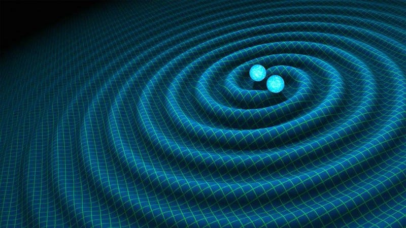
Gravitational waves are ‘ripples’ in space-time caused by some of the most violent and energetic processes in the Universe. Albert Einstein predicted the existence of gravitational waves in 1916 in his general theory of relativity. Einstein’s mathematics showed that massive accelerating objects (such as neutron stars or black holes orbiting each other) would disrupt space-time in such a way that ‘waves’ of undulating space-time would propagate in all directions away from the source. These cosmic ripples would travel at the speed of light, carrying with them information about their origins, as well as clues to the nature of gravity itself.
The strongest gravitational waves are produced by cataclysmic events such as colliding black holes, supernovae (massive stars exploding at the end of their lifetimes), and colliding neutron stars. Other waves are predicted to be caused by the rotation of neutron stars that are not perfect spheres, and possibly even the remnants of gravitational radiation created by the Big Bang.
On September 14, 2015, for the very first time, LIGO (Laser Interferometer Gravitational-Wave Observatory) physically sensed the undulations in spacetime caused by gravitational waves generated by two colliding black holes 1.3 billion light-years away. LIGO’s discovery will go down in history as one of humanity’s greatest scientific achievements.
While the processes that generate gravitational waves can be extremely violent and destructive, by the time the waves reach Earth they are thousands of billions of times smaller! In fact, by the time gravitational waves from LIGO’s first detection reached us, the amount of space-time wobbling they generated was 1000 times smaller than the nucleus of an atom! Such inconceivably small measurements are what LIGO was designed to make.
Gravitational-wave data analysis employs many of the standard tools of time-series analysis. With some exceptions, the majority of gravitational wave data analysis is performed in the frequency domain.
Data from gravitational wave detectors are recorded as time series that include contributions from myriad noise sources in addition to any gravitational wave signals. When regularly sampled data are available, such as for ground-based and future space-based interferometers, analyses are typically performed in the frequency domain, where stationary (time-invariant) noise processes can be modeled very efficiently.
As shown by Einstein himself, the General Relativity Theory of Gravitation allows for wave-like solutions which are generated by accelerated mass motion (or, more generally, by energy-momentum tensor as should be for a relativistic theory).

Measuring Gravitational waves
Gravitational waves cause space itself to stretch in one direction and simultaneously compress in a perpendicular direction.
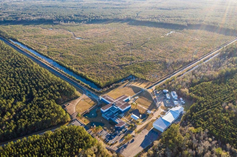
LIGO’s interferometers are set up so that, as long as the arms don’t change the length (4 km physically, 1120 km effectively) while the laser beams (750 kilowatts) are traveling, nothing reaches the photodetector. Otherwise, when something (gravitational waves) happens to change the distance, then the interference pattern can be used to calculate precisely how much change in length occurred. And that change in arm length caused by a gravitational wave can be as small as 1/10,000th the width of a proton (that’s 10^-19 m)!
To get an idea of the data size here, LIGO (the world’s largest gravitational wave observatory) is able to record them extremely precisely. Currently, the data archive holds over 4.5 Petabytes of data. It is expected to grow at a rate of 800 terabytes per year.
Sources of Noise in Gravitational Waves Signal data and how Data Science can help
Noise of non-astrophysical origin contaminates data taken by LIGO. The sensitivity of advanced gravitational-wave detectors will be limited by multiple sources of noise from the hardware subsystems and the environment. The low frequency sensitivity of the detectors (10 Hz) will be limited by the effects of seismic noise. Thermal noise due to Brownian motion will be the most dominant noise source in the most sensitive frequency range of the instruments. At frequencies higher than ∼150 Hz, shot noise, due to quantum uncertainties in the laser light, is expected to be the dominant noise source. Instrumental and environmental disturbances can also produce non-astrophysical triggers in science data, so called ‘glitches,’ as well as increasing the false alarm rate of searches and producing a decrease in the detectors’ duty cycles. The non-Gaussian and nonstationary nature of advanced detector noise may produce glitches, which could affect the sensitivity of searches and be mistaken as gravitational-wave detections, in particular for unmodelled sources.
I quote from this paper named “Efficient Gravitational-wave Glitch Identification from Environmental Data Through Machine Learning”
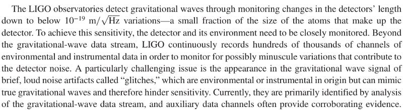
The paper goes on to say, Modern interferometric gravitational-wave (GW) detectors are highly complex and sensitive instruments. Each detector is sensitive not only to gravitational radiation, but also to noise from sources including the physical environment, seismic activity, and complications in the detector itself. The output data of these detectors is therefore also highly complex. In addition to the desired signal, the GW data stream contains sharp lines in its noise spectrum and non-Gaussian transients, or “glitches,” that are not astrophysical in origin. Instrumental artifacts in the GW data stream can be mistaken for short-duration, unmodeled GW events, and noisy data can also decrease the confidence in compact binary detections, sometimes by orders of magnitude
Understanding the noise is crucial to detecting gravitational wave signals and inferring the properties of the astrophysical sources that generate them. Improper modeling of the noise can result in the significance of an event being incorrectly estimated, and to systematic biases in the parameter estimation.
And so in this Kaggle Competition the time series train and test datasets that are given, contain either detector noise or detector noise plus a simulated gravitational wave signal. The task is to identify when a signal is present in the data (target=1)
Understanding fundamentals of Digital Signal Processing
Few basic definitions of periodic waves that are important for this competition:
Amplitude is the height of a wave, the maximum displacement measured from the equilibrium position
Period measures the number of seconds per each cycle
Frequency is the reverse of period, it counts how many cycles can fit in a second. The unit of frequency is Hertz, for example 10 cycles per second = 10 Hertz
Wavelength measures how far a wave has travelled after 1 period (1 cycle). This can be for example the distance between 2 neighboring peaks.
Velocity tells us how quickly a wave is moving to the right. Velocity equals distance over time, so we can say V = wavelength / period = wavelength * frequency
Time Domain vs Frequency Domain Analysis of Digital Signals
A Time domain analysis is an analysis of physical signals, mathematical functions, or time series of economic or environmental data, in reference to time. Also, in the time domain, the signal or function’s value is understood for all real numbers at various separate instances in the case of discrete-time or the case of continuous-time. Furthermore, an oscilloscope is a tool commonly used to see real-world signals in the time domain.
Moreover, a time-domain graph can show how a signal changes with time.
In Frequency domain, your model/system is analyzed according to it’s response for different frequencies. How much of the signal lie in different frequency range. Theoretically signals are composed of many sinusoidal signals with different frequencies (Fourier series), like triangle signal, its actually composed of infinite sinusoidal signal (fundamental and odd harmonics frequencies).
We can move from time-domain to frequency domain with the help of Fourier transform. The Fourier transform can be powerful in understanding everyday signals and troubleshooting errors in signals. Essentially, it takes a signal and breaks it down into sine waves of different amplitudes and frequencies. Fourier’s theorem states that any waveform in the time domain can be represented by the weighted sum of sines and cosines. The frequency-domain shows the voltages present at varying frequencies. It is a different way to look at the same signal.
Why do you actually care to transform time domain to frequency domain?
Because if you can construct a signal using sines, you can also deconstruct signals into sines. Once a signal is deconstructed, you can then see and analyze the different frequencies that are present in the original signal. Take a look at a few examples where being able to deconstruct a signal has proven useful:
■ If you deconstruct radio waves, you can choose which particular frequency–or station–you want to listen to.
■ If you deconstruct audio waves into different frequencies such as bass and treble, you can alter the tones or frequencies to boost certain sounds to remove unwanted noise.
■ If you deconstruct earthquake vibrations of varying speeds and strengths, you can optimize building designs to avoid the strongest vibrations.
■ If you deconstruct computer data, you can ignore the least important frequencies and lead to more compact representations in memory, otherwise known as file compression.
That's some of the absolute basics we need to start on this Kaggle Challenge, and in my next part we will do the Data Preprocessing and analytics part.
My YouTube Video Explaining the model building for Kaggle Submission for the Gravitational Wave Competition.
Literature Survey
Machine Learning Gravitational Waves from Binary Black Hole Mergers
Improving significance of binary black hole mergers in Advanced LIGO data using deep learning
https://iphysresearch.github.io/Survey4GWML/ — a massive collection of papers and other resources related to G-Waves analysis, detection, and more using ML.
Here is a paper that might offer some good background for this competition: Properties of the Binary Black Hole Merger GW150914 https://arxiv.org/abs/1602.03840
Accelerating Recurrent Neural Networks for Gravitational Wave Experiments — This paper presents novel reconfigurable architectures for reducing the latency of recurrent neural networks (RNNs) that are used for detecting gravitational waves.
Inference with finite time series: Observing the gravitational Universe through windows.
A guide to LIGO-Virgo detector noise and extraction of transient gravitational-wave signals