ML Case-study Interview Question: Thompson Sampling for Adaptive Marketing Budget Allocation and Profit Maximization

Browse all the ML Case-Studies here.

Case-Study question

A major online platform invests large budgets in paid marketing campaigns to acquire and retain users. They want to determine how best to allocate these budgets across different campaigns and cost-per-action (CPA) targets. Their past data is confounded by strategic bidding decisions around seasonal events and competitor activities, so simple observational analysis would mislead them. Design an adaptive experimentation framework to identify the optimal marketing action that maximizes the organization’s profit-based objective function (Return - Cost). Propose your approach, outline the modeling choices, explain how you would handle exploration vs. exploitation, and discuss how you would iterate on this system in production.

Detailed Solution

Core Idea

Use adaptive experimentation (multi-armed bandits) instead of relying solely on historical observational data. Randomly perturb the chosen marketing actions (like CPA bids) to generate exogenous variation and estimate the true performance curves for each campaign. Incorporate these learnings into a loop of continuous model updates, then select actions that best trade off exploration and exploitation.

Experiment Design

Introduce a controlled level of randomness in marketing actions. Split your campaigns into different experimental arms that each correspond to a targeted CPA bid range. Randomize these arms over time. This ensures that confounding factors like seasonality and competitor behavior do not bias your estimates.

Causal Estimation

Use inverse-propensity weighting (IPW) to correct for the bias that arises when the system increasingly favors actions that appear optimal. Weight each observation by the inverse of its probability of being chosen. This recovers an unbiased estimate of the average outcome at each action.

Performance Curve Modeling

Fit a parametric function that maps marketing action (for instance, CPA target) to expected profit (Return - Cost). Enforce structural constraints such as the curve crossing zero at zero spend. A convenient choice is a Beta-distribution-based curve because it captures many hump-shaped relationships. The probability density function for the Beta distribution with parameters alpha and beta is:

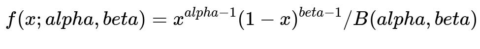
where x is a value between 0 and 1, alpha > 0, beta > 0, and B(alpha,beta) is the Beta function. In your scenario, x can be a scaled version of the marketing action. The posterior distribution over these parameters captures uncertainty.

Explore-Exploit Algorithm

Use Thompson Sampling. Draw a sample from the posterior distribution of the parameters, assume that sample is true, pick the CPA bid that maximizes expected profit for that sampled curve, then observe the outcome. Update the model with the new data. Repeat at each time interval. This adaptively shifts from exploration (due to parameter uncertainty) to exploitation (once estimates converge).

Example Python Snippet

import numpy as np
import pymc as pm

# Suppose we store historical data: actions (x), outcomes (profit),
# and action propensities (p), for inverse-propensity weighting.

x_data = np.array([...])  # Observed marketing actions
profit_data = np.array([...])  # Observed profit for each action
propensity_data = np.array([...])  # Probability of choosing each action

with pm.Model() as model:
    alpha = pm.HalfNormal('alpha', sigma=1)
    beta = pm.HalfNormal('beta', sigma=1)

    # Expected profit as a parametric Beta-based function
    # For illustration, assume x_data is scaled to (0,1)
    # Then map Beta pdf or a related shape to expected profit
    # This is a conceptual placeholder, as real usage might differ

    # Weighted likelihood
    mu = <some_function_of_alpha_beta_that_maps_x_data_to_profit>
    # In real usage, might model profit with normal or other suitable distribution
    sigma = pm.Exponential('sigma', lam=1)
    pm.Normal('obs', mu=mu, sigma=sigma, observed=profit_data,
              total_size=len(profit_data),
              weights=1/propensity_data)

    trace = pm.sample(draws=2000, tune=1000)

# Next step: Thompson sampling action selection
samples_alpha = trace['alpha']
samples_beta = trace['beta']

# Generate the next action for each campaign
def thompson_sample_action():
    idx = np.random.randint(len(samples_alpha))
    alpha_samp = samples_alpha[idx]
    beta_samp = samples_beta[idx]
    # Evaluate expected profit curve with these sampled parameters
    # Then choose the CPA that maximizes profit
    best_action = <argmax_over_possible_actions>
    return best_action

This code repeatedly updates your Bayesian model with new data, using IPW in the likelihood by weighting each observation’s contribution. Then Thompson Sampling picks the next action.

Iteration in Production

The system updates performance curve estimates in discrete rounds. Each round uses the latest data to refine the posterior distribution. The next round’s actions are partly random (to maintain exploration). Over time, the fraction of exploration shrinks if the model gains confidence.

Common Follow-Up Questions

How do you decide how much randomization to introduce at each step?

Adaptive bandits vary the randomization automatically. Thompson Sampling accomplishes this by sampling parameter values from the posterior. When uncertainty is high, the algorithm explores more because different samples produce different recommended actions. As uncertainty shrinks, the sampled parameters converge to similar values, leading to smaller perturbations around the best-known action.

What if the Beta parametric form is too restrictive for some campaigns?

Use more flexible models like Gaussian Process regression. This can model complex shapes that do not follow a single parametric family. You can still maintain a posterior distribution over functions. Implementation is more complex. Many teams start with a simpler parametric form for reliability and speed, then switch to nonparametric models once the simpler method shows limitations.

How do you handle seasonality or sudden external changes?

Retrain the model frequently with the latest data. Keep track of a rolling window or apply decay to older observations. The inverse-propensity weights remain valid as long as your randomization probabilities were accurate. If a sudden shift invalidates older data, favor more recent experiments or re-initialize model parameters.

How would you compare this adaptive system to a standard A/B test?

Standard A/B tests usually allocate fixed percentages to each variant. This gives unbiased estimates for each arm but can waste budget on suboptimal arms. Adaptive methods gradually shift allocation to better arms while still reserving some allocation for exploration. This accelerates learning and reduces regret.

How do you quantify the gains from this system?

Run a smaller, standard A/B test comparing the bandit-driven strategy against your legacy approach. Estimate total profit over a predetermined period. Evaluate variance, average daily returns, or other business-relevant metrics. The bandit approach typically shows higher cumulative reward.

Why is inverse-propensity weighting necessary if Thompson Sampling already introduces randomness?

Thompson Sampling’s randomness skews toward promising actions. Observed outcomes then become biased toward actions that appeared good at the time. IPW corrects this by up-weighting outcomes from less-probable actions, restoring unbiasedness. Without IPW, the parameter estimation can misinterpret systematically under-sampled actions, distorting the performance curve.

How do you ensure that the model remains stable in production?

Validate each new update. Check for abrupt changes in parameter estimates. Have safe fallback CPA actions. Monitor metrics for exploration rates, average returns, and the shape of the predicted performance curves. If the model drifts erratically, investigate anomalies or consider reducing the window of historical data used for training.

What if data is sparse for certain campaigns?

Pool data across similar campaigns if it is appropriate to assume shared patterns. Apply hierarchical or multi-level models. These approaches let campaigns borrow statistical strength from each other. If campaigns differ too much, you might segment them to avoid mixing unrelated data.

Could we apply the same approach to non-marketing scenarios?

Yes. Anywhere you seek to optimize an action based on uncertain payoff. Examples include dynamic pricing, content recommendation, or supply chain logistics. The same bandit-based adaptive experimentation approach helps discover what works best while controlling risk.

---