ML Case-study Interview Question: Two-Layer Ensemble Model for Progressive Daily Sales Opportunity Prioritization
Browse all the ML Case-Studies here.
Case-Study question
A global organization needs an efficient daily prioritization strategy for sales opportunities that remain in an active pipeline for multiple days. The company wants a data-driven model that can capture both static attributes when an opportunity first enters the pipeline and dynamic attributes (like daily contact attempts and number of days in the pipeline). Design a machine learning framework that generates a progressive propensity score daily and helps the sales team prioritize which opportunities to work on each day. Explain how you would structure this two-layer modeling approach, which algorithms you might use, what features you would include, and how you would evaluate model performance.
Detailed Solution
Opportunities may have stable features that never change over time, such as product category or region, and dynamic features that vary daily, such as time in pipeline or number of contact attempts. The two-layer ensemble classifier addresses this by separating static and dynamic attributes:
Layer 1 runs once when the opportunity first appears. It focuses on static features. It outputs an initial propensity score. Layer 2 runs daily (or on any schedule) and consumes both that initial score and the evolving features. It outputs the current daily propensity score, which indicates how likely an opportunity is to close on that day.
Layer 1: GBM Classifier Gradient Boosting Machine (GBM) fits well when learning complex relationships among static features such as product line, initial lead source, or territory. It produces a numeric score that represents the baseline probability of closure. This numeric output is later combined with time-varying attributes in Layer 2.
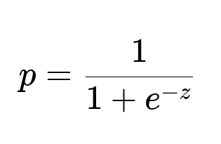
Layer 2: Logistic Regression This layer refines the baseline score using updated features like elapsed days, failed contact attempts, or pipeline stage. The logistic model interprets how newly updated signals interact with the original baseline score from Layer 1. Strongly negative coefficients can diminish the initial score if an opportunity stays in the pipeline for too long, while positive coefficients can reinforce the score if new evidence suggests higher closing potential.
Below, p is the probability that the opportunity closes on the current day, z = w0 + w1 * (Layer1_score) + w2 * (days_in_pipeline) + w3 * (contact_attempts) + ... . Each w is learned during training, and the sign and magnitude of w indicate how each feature contributes to the predicted probability.
Daily Prediction New data for each opportunity flows into Layer 2, which applies the logistic regression to produce the up-to-date propensity score. A threshold or rank ordering approach then prioritizes the daily work list.
Evaluation Historical records of closed or lost opportunities enable model back-testing. Compare cumulative gains curves or average precision on a test set. The two-layer method typically achieves better cumulative gains than a one-shot static model because it leverages new data daily.
Follow-up Questions
1) How would you handle imbalanced class distributions when only a small portion of opportunities eventually close?
Sampling techniques like SMOTE or undersampling can rebalance training data. Adjusting class weights is also common. If the closed class is rare, setting higher class weight for positives can improve recall without drastically inflating false positives. Monitoring metrics like AUC-PR (Area Under Precision-Recall Curve) helps confirm that the model is learning properly. When training the first GBM layer, set the pos_weight parameter or sample from the negative class less frequently. For the second logistic layer, set class_weight="balanced" or manually configure weighting to ensure the minority class is not ignored.
2) How would you deal with the cold start scenario for the second layer if there are not many historical examples of opportunities with dynamic data?
Train both layers on historical pipelines where time-varying attributes are recorded at multiple points. Even if the dataset is small initially, partial fit or incremental learning can be applied for the second layer. Techniques like regularization ensure the model remains stable with limited data. Frequent retraining schedules (for example, weekly or monthly) incorporate newly closed outcomes, improving the model’s understanding of dynamic attributes.
3) How would you update the model on a daily basis given that the pipeline changes frequently?
A daily workflow can run automatically. It collects the latest updates, scores each opportunity using the first layer score (stored from creation time) and the current dynamic features, and outputs a new propensity. Periodically, the model is retrained with fresh labels. Retraining might occur monthly to balance computational cost with model freshness. Online or incremental learning is an option for logistic regression if daily full retrains are expensive.
4) How would you address the interpretability of the second layer’s predictions when stakeholders need justification for daily prioritization?
Layer 2’s logistic regression coefficients highlight which dynamic features raise or lower the final score. For instance, a large positive coefficient on “recent high engagement” feature indicates a strong positive contribution. A negative coefficient on “days_in_pipeline” indicates that lingering opportunities are less likely to close. Showing these coefficients to stakeholders clarifies why the model is pushing some opportunities to the top of the queue.
5) Why not just train a single large model that ingests both static and dynamic features all at once?
A single large model re-evaluated daily on the entire feature set can be computationally heavier, especially if static features are high-dimensional. The ensemble splits the workload: the first layer handles static attributes once, reducing redundant computation. The second layer is a lighter model focused on daily updates. This keeps the framework efficient while enabling progressive predictions over time.
6) How would you manage feature drift or concept drift over time if the nature of the pipeline changes?
Monitoring model performance and shift in feature distributions indicates drift. If the baseline probability from Layer 1 becomes misaligned with new market conditions, retrain that layer with more recent data. Similarly, refresh the second layer more frequently if daily attributes change in ways not captured by the older model. Collect feedback on closed or lost opportunities, retrain with the updated distributions, and track performance metrics to confirm improvements.
7) How would you extend this system to produce not just binary close-or-not predictions but also estimated closure time?
Consider a survival analysis model or time-to-event method that predicts how many days remain before closing. The second layer can be replaced or augmented with survival models that handle censored data. Alternatively, a multi-task approach uses regression to estimate days until closure and classification to estimate the chance of ever closing. The daily pipeline updates can feed into parametric or non-parametric survival techniques that incorporate each day’s dynamic data to update the hazard function.
8) How do you scale this solution if you have millions of daily opportunities?
The first layer runs once per opportunity. That step is less frequent. The second layer must be efficient, so logistic regression is often chosen for speed. Distributed training with Spark or similar frameworks can manage large data volumes. Data streaming infrastructure captures real-time updates. The pipeline can be orchestrated with a daily or near-real-time batch job that scores all open opportunities in parallel.
9) Could you apply this two-layer design to other use cases with progressive dynamics?
Any system where an entity’s probability of conversion changes over time can benefit. Loan applications, subscription renewals, or claims processing share the need for daily updates. The first layer captures the static traits of the entity, while the second layer adjusts for evolving context. The principle of combining a static classifier with a dynamic one is not domain-specific.
10) How would you evaluate whether the second layer truly provides incremental value over a classic single-layer solution?
Compare the performance of the two-layer approach against a baseline single-layer model that uses all features. Conduct back-tests on historical data and measure the lift in metrics like precision at k, recall at k, or the cumulative gains curve. Demonstrate that the second layer consistently outperforms the single-layer approach by incorporating time-varying signals and refining the daily propensity score.


