
ML Case-study Interview Question: Predicting Loan Defaults: A Cost-Sensitive Approach Using Reject Inference

Case-Study question
You are tasked with building a small-business loan approval model that decides whether to approve or reject loan applications based on whether the applicant is likely to default. The outcome is binary: either the loan is fully paid or it defaults, with no partial repayments. You produce a model that outputs a probability of default. You then set a threshold to classify applications as high default risk or low default risk.
The Company wants to know which evaluation metrics you would use, how you would handle false positives versus false negatives, how you would account for sampling bias if your training data only contains previously approved loans, and how you would manage potential anomalies or uncertain cases. They also want to see how you would validate any improved model against a baseline, even though long repayment periods make direct A/B testing tricky.
Explain how you would propose a solution. Discuss your choice of metrics, your approach to thresholding, how you would incorporate reject inference, how you might add anomaly detection, and how you would run or simulate an A/B test. Show how you would handle manual review for borderline cases. Also outline how you would measure success in a real-world scenario that involves cost trade-offs, including differences between missed opportunities (false positives) and actual write-offs (false negatives).
In-Depth Solution
Model Objective
The goal is to predict whether an applicant will default on a requested loan. The model outputs a probability of default for each application. Approving the loan if this probability is below a threshold leads to a classification of “not likely to default.” Rejecting the loan if it is above that threshold leads to a classification of “likely to default.” This is a classification problem with an imbalanced dataset, because only a small fraction of loans typically default.
Choice of Metrics
Precision, recall, and their trade-off are the most relevant metrics. Accuracy is misleading for highly imbalanced data. A high recall ensures the model catches most of the high-risk loans, reducing defaults. A high precision ensures that, when the model flags an applicant as likely to default, it is correct most of the time.
Cost Trade-offs
A false positive is an application rejected when it would have repaid successfully. The loss is the missed interest revenue. A false negative is an application approved when it actually defaults. The loss is the entire principal. If the interest rate is around 10 percent, the ratio of loss from a false negative to a false positive can be about 10 to 1. The threshold can be tuned to minimize total cost. A weighted precision-recall curve can help find the optimal threshold.
Manual Review and Tiered System
Uncertain cases occur when probabilities are borderline. A tiered system uses automated classification for clear approvals or rejections and flags borderline cases for human review. This helps avoid costly mistakes but introduces human labor costs. The number of borderline loans must be tracked to ensure human resources are used efficiently.
Sampling Bias and Reject Inference
Training data usually only covers loans that were actually granted, which can bias the model. Reject inference uses rejected applications in a secondary model. That secondary model estimates default probabilities for previously rejected loans. Combining both models helps reduce bias. This technique is common in credit risk modeling to better represent the real distribution of loan outcomes.
Anomaly Detection
Some defaults defy historical patterns. Monitoring anomalies can highlight unusual behavior in real time. Large feature spaces can trigger many false alarms because of the curse of dimensionality. The anomaly detector flags unexpected patterns, prompting further checks before final approval. This is not a primary classifier but a safety layer.
Model Validation
Direct A/B testing is hard because loans take a long time to repay. An offline evaluation compares new and old models on historical data. A/B tests can still be done in a limited way, but the sample must be tracked for a sufficient period. It is common to rely on offline metrics and partial A/B tests for early signals.
Example of a Probabilistic Classifier
Below is a typical logistic prediction function:
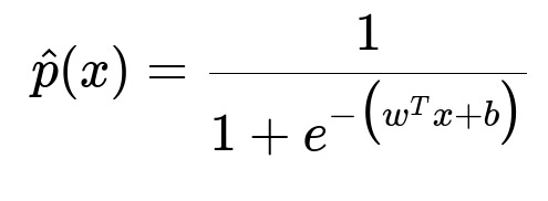
Here w is the weight vector, b is the bias term, and x is the feature vector of the applicant. The probability output by this function is compared to the chosen threshold to decide whether to approve or reject the loan.
Offline vs. Online Testing
Offline testing compares metrics like recall, precision, or profit estimates on historical data with known outcomes. Online testing would assign different subsets of applicants to the new model or the baseline. The company would then measure differences in default rates and profit. Long repayment cycles require extended test durations or surrogate metrics (short-term repayment behavior) for early feedback.
Action if p-value is Just Above 0.05
If a limited-duration A/B test shows revenue improvement but a p-value of 0.06, running the test longer is wise. Variability can be high due to small sample size or short time windows. Effect size and trends in revenue or default rates matter. Collecting more data or continuing the experiment clarifies the observed difference’s significance.
Potential Follow-up Questions
What are the risks of relying solely on precision and recall?
A single threshold might ignore the profit or loss magnitude. Precision or recall does not directly account for the cost difference between defaults and missed opportunities. Weighted metrics or a cost-sensitive framework is better for real-world profit optimization. A high precision may reject too many good loans. A high recall may accept too many risky loans.
How do we optimize the threshold in a cost-sensitive way?
Define a cost function where cost_false_negative is principal loss and cost_false_positive is missed interest revenue. Calculate total cost = cost_false_negative * FN_count + cost_false_positive * FP_count. Sweep thresholds to see which value minimizes this total cost. This is more practical than optimizing a generic measure like F1 score.
How do we incorporate manual review without overwhelming reviewers?
Choose a band around the threshold, for example probability of default in [0.45, 0.55], and label those cases as borderline. Below 0.45 is an auto-approval, above 0.55 is an auto-rejection. The borderline range is small enough for human staff to manage. The threshold can shift if the ratio of borderline cases becomes too large. This approach reduces the highest-risk manual evaluations while leaving most clear decisions to the model.
What is the impact of reject inference on model complexity?
Reject inference adds an extra layer of modeling. It uses data from rejected applications and some assumptions on how they might have performed had they been accepted. It can improve coverage of possible applicant profiles but introduces model complexity and potential errors in inferred outcomes. Careful cross-validation and robust data-cleaning are needed to handle missing labels for rejected cases.
How do we handle anomalies flagged by the anomaly detector?
Any flagged case can be routed for a deeper risk review. A transaction that deviates significantly from past patterns might signal fraud or hidden risk factors. The large feature space leads to higher false alarms. The manual intervention cost needs to be offset by the potential savings from catching hidden defaulters. Monitoring these alerts in production helps refine thresholds for anomaly detection over time.
How would you handle model drift over time?
Monitor key metrics (default rate, precision, recall, or cost) on an ongoing basis. Changing market conditions can cause drift. Periodically retrain the model with recent data. Watch for distribution shifts in applicant demographics or economic conditions. If performance drops, an incremental or full retraining is triggered.
What are the constraints when trying to do an A/B test for such a long-term outcome?
Loan defaults can take months or years to become clear. By the time you collect outcomes for one version of the model, the economic environment or applicant profile may have changed. Testing smaller interim metrics (like short-term missed payments) is possible, though it may only partially reflect true default risk. Collecting enough samples to achieve statistically significant differences can take a long time. Some teams rely on historical backtesting plus partial prospective A/B tests.
How do you justify shipping a model that has a p-value slightly above 0.05?
Check the magnitude of revenue lift or default reduction. If the economic benefit is large, a borderline p-value should not stop the deployment. Gathering more data can confirm significance. Also check for negative signals like an uptick in default rates in a short time frame. If everything points to an improvement, it might be beneficial to deploy while continuing to monitor performance.