ML Case-study Interview Question: Unified Wide-and-Deep CTR Prediction for Multi-Surface E-commerce Ads

Browse all the ML Case-Studies here.

Case-Study question

A large-scale e-commerce platform wants to unify multiple contextual ad surfaces (for example, Buy-It-Again, Collections, Store Root, Item Details) under one unified click-through-rate prediction model. Each surface has its own unique context (past purchases, store category names, reference item attributes, and so on), and they previously used separate gradient-boosted tree models for each surface. They plan to switch to a single Deep Learning model that can handle high-cardinality features (product ID, user ID, search text) and capture complex interactions across surfaces. How would you architect and train a unified model that can outperform the old separate models, lower operational costs, and ensure scalability for future feature additions and new surfaces?

Provide a thorough solution outline that includes data processing, model architecture, training approach, calibration, and deployment. List potential pitfalls and how you would mitigate them. Propose ways to assess success both offline and in A/B tests.

Detailed solution

A unified model merges training examples from all ad surfaces into one dataset, yielding richer cross-surface user–product interactions and offering more robust model coverage. The unified approach eliminates separate model overhead and simplifies infrastructure. This model uses a Deep Learning framework to incorporate high-cardinality features, handle contextual differences between surfaces, and leverage shallow interactions that capture subtle patterns.

Data generation

All ad impressions come from multiple surfaces. The training pipeline merges them into a single dataset. The data tracks user ID, product ID, product attributes (brand, category, text embeddings), context signals (surface type, reference item attributes, collection names), and historical user behaviors (clicks, purchases). The model treats missing attributes (for surfaces where a given context field does not exist) as default values. This simpler imputation keeps complexity low and is feasible at scale.

Model architecture

A Wide-and-Deep approach, combined with second-order factorization machine interactions, works effectively. The wide side includes lower-cardinality categorical signals (surface type indicators, broad product categories) and continuous features (historical purchase counts, price). The deep side processes high-cardinality embeddings (user ID, product ID, brand text). Then the model adds pairwise feature interactions before the final output layer.

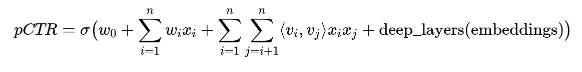
pCTR is the predicted probability of a click. sigma(...) is the logistic function. w_0 is a bias term. w_i is the weight for feature i. x_i is the value of feature i. v_i is the learned embedding vector for feature i. deep_layers(embeddings) are the nonlinear transformations (dense layers) applied to the embedding outputs.

The embeddings reduce large categorical spaces (millions of product IDs or user IDs) into dense vectors. The factorization machine term sum_{i=1 to n} sum_{j=i+1 to n} <v_i, v_j> x_i x_j models second-order interactions. This captures cross-feature effects that standard feed-forward layers alone might underrepresent.

Model training

A classification objective with log loss on click vs. non-click data handles training. Stochastic gradient descent or Adam optimizers work well with large-scale data. Batches mix impressions from all surfaces, forcing the network to learn universal and context-specific patterns. Mean target encoding (MTE) features add historical click rates for user–product or reference–target pairs, boosting performance.

Calibration

Deep models can misrepresent actual probability. Techniques like temperature scaling or isotonic regression can bring predicted pCTR closer to real CTR. This ensures fairer pricing in second-price auctions and more stable bidder behavior. Monitoring calibration metrics (like reliability curves and calibration loss) helps fine-tune this step.

Deployment

A single model replaces multiple older tree-based models. Runtimes improve if the new model is on a modern serving stack with GPU/accelerator support. Feature computation is more centralized. Missing fields remain zero or default-coded. Real-time updates (for user sessions or short-term features) can feed into the same model input in production.

Observed impact

Once deployed, the model can handle all surfaces in one pass, improving coverage and user–product matching. This often raises AUC and lowers log loss, boosting incremental product sales for advertisers and relevance for users. Real-time or frequent feature refreshes push further gains.

Potential pitfalls

Data leakage can occur if features that do not exist in real time slip into training. Thorough data validation is critical. Large embedding tables risk memory blow-ups, so dimension sizes must be chosen carefully. Overfitting is possible with massive model capacity, so regularization or dropout are important. Thorough offline checks (AUC, log loss, calibration) and online A/B tests track actual business metrics (CTR, conversions, revenue).

Example code snippet

import tensorflow as tf
from tensorflow.keras import layers

# Simple wide-and-deep with factorization machine snippet
class FactorizationMachineLayer(layers.Layer):
    def __init__(self, k):
        super().__init__()
        self.k = k

    def call(self, x):
        # x is (batch_size, num_features)
        sum_of_squares = tf.square(tf.reduce_sum(x, axis=1))
        square_of_sums = tf.reduce_sum(tf.square(x), axis=1)
        second_order = 0.5 * (sum_of_squares - square_of_sums)
        return tf.expand_dims(second_order, axis=1)

# Wide side input
wide_inputs = tf.keras.Input(shape=(num_wide_features,), name="wide_inputs")

# Embeddings for deep side
embed_inputs = tf.keras.Input(shape=(num_embed_features,), name="embed_inputs")

# Factorization machine second-order interactions
fm_layer = FactorizationMachineLayer(k=embedding_dim)(embed_inputs)

# Deep side fully connected layers
x = layers.Dense(128, activation='relu')(embed_inputs)
x = layers.Dense(64, activation='relu')(x)

# Concatenate wide side, second-order interactions, and deep outputs
combined = layers.Concatenate()([wide_inputs, fm_layer, x])
output = layers.Dense(1, activation='sigmoid')(combined)

model = tf.keras.Model(inputs=[wide_inputs, embed_inputs], outputs=output)
model.compile(optimizer='adam', loss='binary_crossentropy')

This shows a rough structure. In practice, you add embedding lookups or text encoders for brand names, product IDs, user IDs, then feed them into the deep side.

Follow-up question 1: Why unify models for multiple surfaces instead of training separate models?

Unifying reduces operational complexity. A single model has fewer pipelines and updates, simplifying monitoring and reducing overhead. Combined data from multiple surfaces exposes shared user–product features. A user’s click behavior on one surface informs predictions on another. Unifying also avoids repeating engineering work for each new surface. This synergy boosts predictive power and aligns future expansions under one pipeline.

Follow-up question 2: How do you avoid performance loss from missing context fields?

Missing fields reflect absent context (for example, a user might not have a reference product in certain surfaces). Simple default encoding (like zeros or special tokens) works at scale. The model sees these defaults frequently during training, thus learning to interpret them. Higher-capacity deep models can capture “missingness” and adjust predictions accordingly. This approach is easier than advanced imputation, which can be slow or infeasible for large data streams.

Follow-up question 3: Why add shallow factorization machine interactions on top of a deep network?

Second-order interactions help the model capture explicit pairwise feature patterns that might get blurred in purely deep layers. This can significantly boost performance when certain cross-feature combinations (for example, user segment with brand category) are highly predictive. Deep layers can learn complex representations, but an explicit factorization machine term ensures direct modeling of pairwise interactions without relying solely on deeper nonlinear transformations.

Follow-up question 4: How do you ensure your unified model stays well-calibrated?

Monitor calibration metrics after training. Techniques like temperature scaling adjust the final logits by a scalar factor, aligning predicted probabilities to actual click frequencies. Isotonic regression is another approach that fits a piecewise function mapping raw predictions to probability space. Re-check calibration in offline holdouts and in production logs. Keep an eye on drift if user behavior changes over time.

Follow-up question 5: How do you prevent overfitting with so many parameters?

Large-scale data helps, but regularization (L2, dropout, or embedding dimensional constraints) is still critical. Embedding dimensions should not exceed what is needed for the training set size. Layer normalization or batch normalization can stabilize training. Early stopping with validation data is common, and cyclical or decaying learning rates help the model converge without overfitting.

Follow-up question 6: How do you measure success in production?

Offline measures: AUC, log loss, and calibration on holdout sets. Online measures: CTR, conversion, cart adds, and advertiser return on ad spend (ROAS). A/B testing with user cohorts is standard. Compare the new model to the baseline. Watch for improvements or declines in user engagement, conversions, or advertiser metrics. Log relevant signals for debugging. Then scale up once confident in stable gains.

---