
ML Case-study Interview Question: XGBoost Ranking for Hybrid Recommendations: Combining Content & Collaborative Signals at Scale


Browse all the ML Case-Studies here.
Case-Study question
You have a massive user-item interaction platform that surfaces business recommendations to tens of millions of users. Past approaches used a matrix factorization model that computed user vectors and business vectors, then performed a dot-product to generate top-k recommendations. Many users with sparse activity were excluded because they had too few interactions. The system also could not incorporate content-based features (like text embeddings, business ratings, or user segments). Propose a new recommendation pipeline that handles both head and tail users. Describe how you would (1) combine collaborative filtering signals with richer content-based features, (2) define a training objective that ranks relevant businesses higher than less relevant ones, (3) handle the need for negative sampling, and (4) scale the system to millions of users. Explain every design choice and detail each step in your solution.
Proposed Solution
Matrix factorization alone provides user embeddings and business embeddings but fails on users with few interactions. Enriching signals with content-based features (business categories, review text embeddings, user metadata) addresses the cold-start problem. Training a supervised model on top of these signals combines the best of both worlds.
Using an XGBoost ranker is an efficient solution. XGBoost handles multiple features, offers tree-based explainability, and scales well. Defining the objective as a ranking metric ensures the model learns to prioritize businesses that users will engage with. Normalized Discounted Cumulative Gain (NDCG) is a suitable metric for this because it prioritizes relevant items near the top of recommendations.
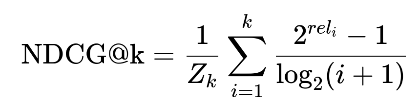
Here Z_k is a normalizing constant so that the ideal ranking has NDCG@k = 1.0. rel_i is the relevance score for the business at rank i. The rank index is i. The term 2^{rel_i} - 1 ensures higher relevance gains more weight, while log_2(i+1) discounts items at lower ranks.
Defining groups for LambdaMART training requires grouping by user and location so pairwise comparisons are performed on relevant sets of items. Content-based features include text-based similarity computed by encoding business reviews with a universal sentence encoder, aggregating them at the business level, and further aggregating user embeddings from the businesses they have interacted with. A cosine similarity between these representations gives a vital signal, especially for users with fewer interactions.
Controlling negative sampling is crucial. Generating implicit negatives by considering businesses a user never interacted with can introduce bias from how items were presented in the past. A recall step that filters businesses by popularity or user location reduces sampling noise and ensures training data remains representative of real-world serving conditions.
Scaling predictions demands a second recall stage at inference time. Narrowing the candidate pool by restricting distance or category constraints reduces the number of user-business pairs, making feature computation and XGBoost scoring more tractable.
Explanation of Each Technology and Approach
XGBoost ranker learns a function that maps each user-business pair to a relevance score. The rank:ndcg objective ensures that pairs with higher actual engagement probabilities appear higher in the ordering. This approach efficiently leverages both collaborative and content-based signals.
Matrix factorization outputs remain valuable. Including dot-product scores from user and business embeddings (trained previously on large interaction data) serves as a robust collaborative signal. Content signals such as text similarities fill in knowledge for sparse users. The combination handles both users with substantial histories and those new or sporadic.
Aggregating embeddings from text reviews captures semantic nuances about businesses. Summarizing what businesses offer, and matching these summaries to user interests, bridges the cold-start gap. This representation also helps for users who only rated a few businesses but wrote or consumed text-based content.
Negative sampling can distort training if done blindly. Restricting negatives to a recall step, such as retrieving top candidates from matrix factorization or popularity, ensures the training process sees realistic user-business pairs. This approach aligns well with how recommendations are eventually surfaced.
Follow-Up Questions and Detailed Answers
How do you ensure that the cold-start user segment still gets meaningful recommendations without sacrificing the performance of head users?
Tail users lack sufficient interaction data. Relying on content-based features like user demographics (if available), business category preferences, or text-based similarities helps bridge this gap. The model sees a limited collaborative signal for tail users but a strong content signal if the text embeddings match user traits. The learning algorithm balances the weighting of each feature by maximizing the rank-based objective. Tree-based splits in XGBoost typically shift more weight toward content signals when interaction data is scarce. This does not hurt head users because they retain strong collaborative signals. The model automatically discriminates which features reduce ranking loss for each user.
How do you define relevance levels for the ranking objective when interactions vary in strength?
Relevance levels match engagement intent. Views might be a lower-intent action, while bookmarks or orders are stronger. A standard approach is to assign integer gains like 1 for views, 2 for bookmarks, 3 for highly active behaviors, and so forth. NDCG uses these to weigh items. The model sees higher gains for interactions that reflect stronger user interest and learns to rank these items toward the top.
How do you debug or interpret the model if it relies on many features?
Tree-based methods allow feature importance extraction. XGBoost logs importance by total gain or split count. Partial dependence plots show how changing one feature alters the predicted relevance while holding others constant. Examining the distribution of predicted scores for various user segments clarifies whether the model is overfitting or ignoring key signals. If partial dependence indicates the model under-weights collaborative signals, it may need more negative samples from the dot-product top-k. If text-based signals dominate for all users, the hyperparameters or negative sampling strategy might need tuning.
How do you handle biases introduced by negative sampling in a large-scale setting?
Bias often appears if the sampled negatives do not match how a user interacts in production. Random negatives might ignore the fact that certain users are rarely exposed to specific businesses. Restricting negatives to a realistic recall set (such as location-based candidates or top-K popular items) ensures the training set aligns with how the system surfaces items. Re-sampling multiple times can help. Another approach is weighting negative instances so the class ratio approximates real-world engagement. XGBoost can handle these sample weights. A consistent recall strategy at inference time ensures alignment with training distribution.
How do you scale the inference pipeline to millions of users and businesses?
The first recall pass prunes candidate businesses using location or popularity filters. Only a small subset of businesses remain for each user. Feature computation occurs next. A broadcasting approach or distributed key-based joins can unify user and business features on Spark. Batched XGBoost scoring on these pairs ranks them, and the top-k items are retained. This method prevents a blowup from scoring all possible user-business pairs, which would be infeasible at large scales.
How do you verify that the hybrid model indeed uses both content and collaborative signals correctly?
Comparison of partial dependence plots for key collaborative features (dot-product score) versus content features (text-based similarity) shows how predictions vary. Higher sensitivity for the matrix factorization score indicates the model emphasizes collaborative signals, especially for head users. Stronger sensitivity for the text-based feature indicates content signals matter for users with limited history. Observing both high importance ensures the model balances them for maximum overall performance. Offline metrics like NDCG on test data and online metrics from A/B tests confirm improvements. Checking real recommendations with QA testers or product managers helps verify business alignment.
How do you keep the system maintainable if you add more complex models in the future?
Modular data pipelines isolate feature extraction, negative sampling, and model training. Changing or extending the model is simpler if each part is well-defined. Well-structured data ingestion pipelines let you add new features without rewriting the system. The recall layer remains the same, so only the scoring function changes if you switch to neural networks or hybrid architectures. Detailed documentation of each component ensures future iterations can happen with minimal disruption.
How would you adapt this approach if you wanted to optimize a different business metric, like user retention or average order value?
Training signals must reflect your business metric. If maximizing average order value, assign higher relevance scores to transactions with higher value. Construct your label period to capture interactions that strongly correlate with longer-term retention or monetary value. The ranking approach remains, but the label definitions shift. The pipeline for recall, negative sampling, and XGBoost training still applies. You might adjust hyperparameters or the tree depth if you suspect new features or different label distributions demand a different complexity level.
What if some content-based features are sparse or have high cardinality, like a large set of possible categories?
XGBoost handles sparse features by learning split thresholds that skip empty or rare categories. Combining categories in a text-based embedding can reduce dimensionality. You can store multiple categories or text descriptors in a single learned embedding. The essential idea is to preserve relevant semantic information without creating thousands of one-hot columns. Regularization parameters in XGBoost help manage overfitting from large feature spaces.
What key mistakes might cause an overestimation of improvement when comparing hybrid approaches to matrix factorization?
Mismatched training and test sets can inflate performance. Leakage occurs if the label period overlaps the feature period. This might lead to artificially high NDCG. Failing to use a location-based grouping for the rank objective can mask overfitting to single-city patterns. Another pitfall is ignoring a valid baseline like business popularity for tail users, where matrix factorization alone does not apply. Proper A/B experimentation ensures offline gains translate to real user engagement.
How do you ensure the text-based embedding features do not explode your storage or run-time resources?
Aggregating the embeddings at the business level and then at the user level compresses the textual information into a reasonable dimension (for example, 512 or 256). Storing these representations in a key-value store allows fast lookups at inference time. Distributed systems that broadcast smaller embedding tables avoid transferring massive arrays of raw review text. Offline precomputation of embeddings ensures scoring only requires a vector lookup rather than re-encoding text on the fly.
Why does the model sometimes fail to learn from the collaborative score if you only sample negatives from the dot-product top-K?
All negative examples would appear to have an artificially high collaborative score, making the model see that higher collaborative scores can sometimes mean negatives. This leads to a negative correlation between that score and the label. Diversifying the negative sampling to include random or popularity-based negatives ensures the model encounters pairs with a lower collaborative score. Balancing these sets helps the model recognize that high collaborative scores often indicate relevance.
How do you decide the weighting or trade-off between location relevance and personalization?
Observing partial dependence for location features indicates how strongly distance constraints or local popularity matter. If your product is strictly local, the model might rely on location-based features by design. Tuning XGBoost hyperparameters and data sampling methods can emphasize local signals. Adjusting the group definition so that city-level or region-level grouping is included ensures ranking within a realistic candidate set. Cross-validation on separate geographic splits verifies whether you are overfitting to certain regions.
How do you interpret improvements in MAP or NDCG for a business-oriented stakeholder?
Explaining that MAP quantifies how early in the ranked list the relevant items appear clarifies that users discover what they want faster. NDCG measures the overall ranking quality with heavier weight on top positions. Doubling MAP means relevant items now appear near the top much more often, so a user is more likely to see interesting businesses early. This can improve engagement metrics, revenue from associated transactions, or user satisfaction. Providing real examples of recommendations that improved helps non-technical stakeholders appreciate the significance of the ranking metrics.
What if you want to run different ranking objectives for different user groups?
Segmenting user groups can help. For new users, optimizing higher-level engagement might matter more than deeper actions. For power users, you might want to optimize advanced interactions. Training separate models or multi-task learning can unify these objectives. The pipeline for feature extraction remains the same. The difference is in how you define group IDs and relevance. You can maintain one global model with a feature indicating user segment, or train distinct models and blend them.
How do you handle the risk of data leakage or label contamination?
Splitting data by time prevents features from seeing the outcome. For instance, if you compute features up to time T and labels from time T to T+delta, you avoid direct overlap. Ensuring any new interactions after time T do not feed back into your feature generation pipeline is critical. If the system re-samples negatives with knowledge of the future, the training set might become biased. Carefully partitioning data and checking differences between training, validation, and test sets is essential.
How do you measure the success of your final system in production?
Monitoring changes in click-through rates, conversion rates, or user retention after launching the new hybrid system. A typical approach uses A/B testing: a control group sees matrix-factorization-based recommendations, while a treatment group sees hybrid-based results. Measuring improvements in user actions, session length, or revenue determines how well the new system performs. Stable improvements in these metrics indicate that offline gains translated well in a real environment.