ML Case-study Interview Question: Improving Home Valuation by Mining Listing Texts with Embeddings and Taxonomy Matching.

Browse all the ML Case-Studies here.

Case-Study question

A real-estate listings platform wants to improve its automated home-value model by extracting valuable details from unstructured listing descriptions. Many relevant features, such as specific amenities, remodeling status, or unique upgrades, are buried in free-text listings. Structured databases do not always contain these attributes. Develop a plan to ingest textual descriptions into the valuation model without sacrificing interpretability or performance. Describe how to identify key phrases that correlate with home value, convert them to numeric features, and integrate them into the training pipeline. Explain challenges, design decisions, and approaches to ensure interpretability.

Detailed Solution

Text Embeddings vs. Direct Phrase Extraction

Text embeddings can represent entire listing descriptions as dense vectors. Average word embeddings or model-based document embeddings capture the underlying semantics without manual hand-engineering. This approach often loses interpretability. Direct extraction of key terms through a taxonomy-based structure yields features that are easier to map back to tangible amenities.

Real Estate Taxonomy

A curated hierarchy of real estate terms organizes synonyms under broad categories (for example, “deck,” “yard,” “pool”). Each category has sub-terms (hyponyms) that capture specific features. These sub-terms map back to a parent feature (hypernym) like “exterior attributes.” This lets us label properties consistently, even if the exact phrase in the listing is not a perfect match.

Featurization Pipeline

A natural language processing model (for instance, a fastText-based approach) encodes both the taxonomy terms and each unique listing phrase into semantic vectors. Similar phrases cluster together. A K-nearest neighbors (KNN) step looks for the nearest taxonomy term to the given listing phrase. If the similarity exceeds a chosen threshold, we assign the feature to the property. Proper tuning of this threshold balances capturing real features and avoiding misclassifications.

Similarity Computation

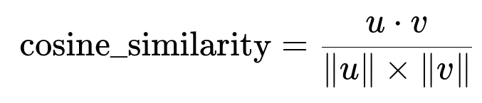
u and v represent embedding vectors of length n. The dot product in the numerator measures alignment. The product of their magnitudes in the denominator normalizes for vector length. Higher scores indicate greater semantic overlap.

Model Integration

Binary flags indicate presence or absence of each amenity. The model then incorporates these flags as additional predictors. Historic data is used for backtesting and ensuring that newly added text-based features reduce errors and bias. This approach maintains interpretability: any flag is directly tied to a human-readable phrase in the listing.

Practical Example

Large backfills on historical listings generate text tags for every home. Each tag is converted to a vector, then matched against taxonomy terms. We store the matches as new columns (e.g., “HasSwimmingPool = 1 or 0,” “HasYard = 1 or 0”). The training set remains consistent with the timeline of property listings to prevent data leaks. Once tested in a backtest framework, stable improvements justify production release.

Production-Ready Considerations

Data pipeline reliability is essential. A continuous feed of new listing descriptions must be processed, matched, and stored. Accuracy depends on frequent retraining or fine-tuning of embeddings to keep up with new terms. Tighter thresholds yield more precision, looser thresholds yield more coverage. Each feature can be validated by analyzing model residuals or distribution shifts.

Possible Follow-Up Questions

How does the presence of subjective phrases (e.g., "luxurious," "spacious") affect the model?

Subjective phrases often increase noise. The taxonomy approach excludes vague terms by focusing on tangible property features (e.g., “granite countertops,” “hardwood floors”). Subjective terms yield unclear signals (one agent’s “spacious” might be another’s “cozy”), so ignoring them can reduce confusion. If these terms appear, building a dedicated filtering step or assigning them lower weights can help.

How do you handle ambiguous or aspirational terms (e.g., "pool table," "tear down")?

Terms referencing a future plan (“tear down to build…”) or different objects (“pool table” vs. “pool”) can lead to misclassification. Training data with these edge cases helps the embedding model learn contextual differences. Tighter similarity thresholds and manual checks on frequent false positives reduce confusion. If the KNN incorrectly maps “pool table” to “swimming pool,” stricter thresholds or refining the taxonomy can fix it.

How do you evaluate the impact of new features on the valuation model?

Running a backtest on historical data is typical. Partition the data by month. Train the model at month-end and evaluate predictions on next-month sales. Compare error metrics, bias metrics, and outlier metrics between control (no new features) and experimental (new text-based features). Statistically significant improvements in error and bias indicate positive impact.

How do you ensure model explainability when text embeddings are used?

Dimensional embeddings are inherently opaque. Directly translating them into discrete features is more transparent. Instead of feeding raw embedding vectors, we create top-level flags (e.g., “HasPool = 1”). Each feature is interpretable. Model outputs can be explained by referencing which phrases were matched in the property’s listing.

Why not rely solely on regular expressions?

Regular expressions require manual enumeration of synonyms and phrases. That approach is cumbersome and prone to missing new terminology. Machine-learned embeddings generalize to variations of key words. Regex might still be useful for specific patterns like invalid addresses or disclaimers, but not for broad concept extraction.

What techniques reduce false positives in KNN matching?

One technique is adjusting the similarity threshold. Another is clustering frequent misclassifications and analyzing their embeddings. Refinements to the taxonomy (grouping or splitting categories) help. Regular audits of the top frequent tags that trigger misclassification also catch anomalies.

How do you handle training data temporal alignment?

We only include listing-based features that were available to the model at that historical date. This prevents lookahead bias. For example, a listing description from 2019 is only used in 2019’s training. A data pipeline ensuring date-correct merges is crucial.

How would you generalize this pipeline to other text domains?

A similar approach applies. First, define a domain-specific taxonomy of relevant attributes. Embed each text snippet with a suitable model. Use a nearest-neighbor or similarity-based classifier to map real text to taxonomy features. Integrate those features into a downstream model. The principle of threshold tuning, interpretability, and pipeline reliability remains the same.

Why is partial usage of embeddings (through nearest-neighbor matching) better for interpretability?

Full embeddings produce continuous, high-dimensional features that are hard to map back to real-world attributes. Nearest-neighbor matching anchors the embeddings to known, interpretable categories. This results in discrete indicators that humans can understand.

What if some properties have no listing descriptions?

Not all listings have textual data. The model can default those features to null or zero. If no text-based features exist, the original structured data features drive the prediction. Model retraining ensures no skew or bias.

Could you show a minimal code snippet using fastText and KNN for term matching?

Yes.

import fasttext
from sklearn.neighbors import NearestNeighbors
import numpy as np

# Load or train your fastText model
# model = fasttext.train_unsupervised('listing_texts.txt')
# For illustration, assume model is already trained

taxonomy_terms = ["pool", "in-ground pool", "heated pool"]
term_vectors = np.array([model.get_word_vector(t) for t in taxonomy_terms])

knn = NearestNeighbors(n_neighbors=1, metric='cosine').fit(term_vectors)

def get_taxonomy_label(tag, similarity_threshold=0.9):
    tag_vec = model.get_word_vector(tag)
    dist, idx = knn.kneighbors([tag_vec], n_neighbors=1)
    # Cosine distance = 1 - cosine_similarity
    sim = 1 - dist[0][0]
    if sim >= similarity_threshold:
        return "pool"  # Or the parent category
    return None

test_tag = "pool oasis"
label = get_taxonomy_label(test_tag, 0.9)
# label is "pool" if similarity >= 0.9, else None

Each tag is embedded, matched, and flagged. Tuning the threshold adjusts classification strictness.

---