ML Case-study Interview Question: Lightweight DCT-Based Blur Classification for Automated Car Image Inspection

Case-Study question

A major used-car marketplace has a computer vision pipeline that processes thousands of car images daily for automated inspection. Some images suffer from blur due to camera shake, dirty lenses, or poor focus, leading to incorrect damage detection. Blurry images that are passed on without verification cause false positives or false negatives in downstream models, resulting in financial and user-experience losses. The company wants a robust blur-classification module that flags these images before any further processing. The system must be fast, lightweight, and accurate. How would you design and implement such a blur-classification system?

Detailed In-Depth Solution

Overview

Blur occurs when edges in an image lose their sharpness. A fast and lightweight method is essential because every image entering the pipeline must be checked. A viable solution involves transforming the image into a frequency domain representation using the Discrete Cosine Transform (DCT), extracting relevant statistics, and training a classifier to detect blurred images.

Step 1: Understanding Blur in Images

Blur diminishes sharp intensity transitions along edges. Clear edges show abrupt pixel value changes. Blurry edges show gradual changes. Excessive blur leads to inaccurate detection of defects or features, harming subsequent models.

Step 2: Using the Discrete Cosine Transform

DCT represents an image as sums of cosines at different frequencies. Most visual information concentrates in a few low-frequency coefficients. This property helps us construct a compact representation of the image’s sharpness profile.

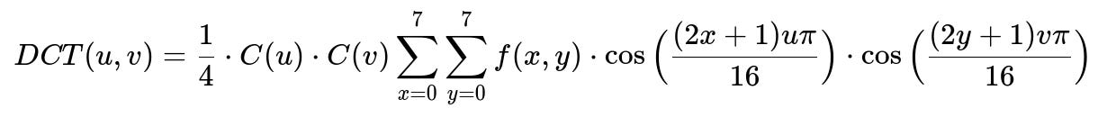
Here:

• f(x,y) is the pixel intensity at spatial coordinates x, y in the 8-by-8 block.

• DCT(u,v) is the transform coefficient at frequencies u, v.

• C(u) and C(v) are scaling factors for u, v frequencies.

Each 8x8 block is converted to its DCT coefficients. We split the resulting 8x8 DCT matrix into low, medium, and high frequency regions. Each region’s statistical measures (mean, variance, kurtosis, skewness, entropy, energy) capture distinct aspects of sharpness or blur.

Step 3: Implementation Details

A Python-based approach uses a small stride to process 8x8 blocks of the image. After applying DCT on each block, compute the statistics. Concatenate these statistics to form an 18-dimensional descriptor (6 statistics per region x 3 regions).

Below is a simplified code snippet illustrating these steps:

import cv2
import numpy as np

def compute_dct_descriptors(img_path):
    B = 8
    img = cv2.imread(img_path)
    img_yuv = cv2.cvtColor(img, cv2.COLOR_BGR2YUV)
    y_channel, _, _ = cv2.split(img_yuv)

    # Extract 8x8 blocks
    stride_blocks = np.lib.stride_tricks.as_strided(
        y_channel,
        shape=(y_channel.shape[0] // B, y_channel.shape[1] // B, B, B),
        strides=(
            y_channel.strides[0] * B * y_channel.shape[1],
            y_channel.strides[1] * B,
            y_channel.strides[0],
            y_channel.strides[1]
        )
    ).reshape(-1, B, B)

    # Apply DCT and compute statistics
    descriptors = []
    for block in stride_blocks:
        dct_block = cv2.dct(np.float32(block))
        # Split DCT block into low, mid, high frequency regions
        # Then compute mean, variance, skewness, kurtosis, entropy, energy for each region
        # Combine features
        # descriptors.append(features_for_this_block)

    # Average feature values across all blocks
    # final_descriptor = np.mean(descriptors, axis=0)
    return np.array(descriptors).mean(axis=0)

# Example usage
# feature_vector = compute_dct_descriptors("car_image.jpg")
# classifier_prediction = blur_classifier.predict([feature_vector])

A gradient boosting or random forest classifier can then label images as “blurred” or “sharp” based on these feature vectors.

Step 4: Model Training and Evaluation

Split a dataset of labeled images into training and validation sets. Train the classifier on the 18-dimensional descriptors per image. Evaluate performance using accuracy, precision, recall, and F1-score. For large images (for example, 1080x1920 resolution), the process remains fast because computing DCT on small blocks is efficient and requires minimal memory usage.

Step 5: Deployment and Use

Embed this module before any image-based damage or defect-detection pipeline. If an image is flagged as “blurred,” discard it or request a better-quality image. This prevents false positives and negatives. The module runs on single-core machines in ~12 milliseconds per image, which is suitable for real-time or near real-time applications.

Follow-up Questions

What is the advantage of DCT over direct pixel-based statistics?

DCT highlights differences in spatial frequency. Direct pixel-based statistics can miss frequency-specific details. DCT-based features retain sharpness information in distinct frequency regions. This helps distinguish blurry edges (which have reduced high-frequency components) from sharp edges.

How do we decide on the threshold for labeling an image as blurred?

The classifier learns this threshold internally through supervised training. Class labels (blurred vs. sharp) guide the decision boundary. If no classifier is used (e.g., a simpler rule-based approach), compute descriptive statistics over high-frequency components and pick a threshold experimentally by validating on a labeled dataset.

Why is this approach preferred over a deep learning model for blur detection?

Deep neural networks are heavier in computation and require extensive training data. DCT-based methods are fast, do not need large training sets for feature extraction, and run efficiently on CPUs. This is crucial because every image must pass through the blur detector.

How do we handle different camera resolutions or aspect ratios?

Resize images to a consistent resolution or maintain block-based processing. Block-based DCT generalizes because each block is always 8x8. Varying image sizes still yield consistent block-level DCT descriptors, which are then averaged.

Is there a risk of missing partial blurriness in certain regions?

Partial blur in small regions can reduce local high-frequency energy. The block-wise approach mitigates this risk because each block is assessed separately. If partial blur is significant, blocks in that region will exhibit different statistics and influence the final feature vector.

What happens if the classifier mislabels a slightly blurred image as sharp?

Slight misclassifications occur. The goal is to keep the false acceptance rate of blurred images low. A mislabeled mildly blurred image might affect downstream tasks. We reduce this risk by training on diverse data, tuning hyperparameters, and monitoring real-world performance.

Why do we split DCT coefficients into low, medium, and high frequency regions?

Low frequencies capture global illumination, medium frequencies capture broader texture details, and high frequencies capture fine edges. Separating them reveals how much detail an image retains in each band. Blurred images lose important high-frequency components.

Could we detect blur by simply applying a Laplacian filter?

Yes, Laplacian-based focus measures are popular. They compute pixel intensity variations directly. DCT-based methods capture a broader spectrum of frequency content in one transform. Both approaches are valid. DCT helps produce a compact descriptor with well-known compression properties.

How would you scale this solution if traffic jumps from thousands of images per day to millions?

Parallelize or distribute the process. Each image’s blur computation is independent. Containerize the solution and run multiple instances behind a load balancer. The lightweight nature of the DCT-based approach ensures linear scaling.

---

Use these explanations and approaches to confidently implement or discuss a robust blur-classification module in a real-world interview setting.

---