
ML Case-study Interview Question: Transformer-Based Demand Forecasting for Fashion with Monotonic Discount Modeling


Browse all the ML Case-Studies here.
Case-Study question
A large online fashion retailer faces a demand forecasting problem for millions of articles. They have a fixed inventory for each article at the start of a season and cannot reorder items. They need a system to forecast how demand will evolve over a 26-week horizon. The solution must account for the impact of discounts on weekly demand in each country. Historical data is short and frequently sparse, with many articles not selling every week. Also, a big portion of the assortment is replaced each season (cold start issue).
They ask you to propose a forecasting model and a corresponding pipeline. They want to incorporate a monotonic relationship between discount and demand, because higher discounts should not result in lower demand. They plan to use a down-stream price optimizer that relies on your discount-dependent forecasts. Show how you would design an end-to-end data science solution, from data preprocessing and modeling all the way to performance monitoring in production.
Detailed Solution
Data Preprocessing
Inventory arrives once at the start of each season, which can cause stock-outs. Observed sales may not match real demand. For each article, sizes can go out of stock and obscure true demand. Estimate missing demand by learning an empirical probability distribution over sizes when all sizes are in stock. Impute unobserved demand if certain sizes are unavailable. Exclude these imputed data points during model evaluation.
Include covariates that provide brand, commodity group, price, discount, stock, stock uplifts (deliveries or returns), etc. Some covariates are only known historically (e.g., actual stock levels), others can be forecast or approximated for the future (e.g., upcoming deliveries), and some never change over time (static features like brand).
Model Architecture
Use a global forecasting model with a transformer-based encoder-decoder. Train one single model on all articles, which helps learn patterns across the full catalog. Split the modeling into two parts: near future (first 5 weeks) and far future (up to 26 weeks).
Encoder processes historical data (demand, discount, other features) and outputs a learned representation. Decoder receives forecast-horizon covariates, plus the encoder’s representation, to predict future demand. Control the discount-demand relationship in a dedicated monotonic demand layer.
Key Distribution Formula
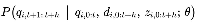
Here:
q_{i,t+1 : t+h} is the demand over the forecast horizon.
q_{i,0:t} is the historical demand.
d_{i,0:t+h} is the applied discount from history into the future.
z_{i,0:t+h} are other covariates.
theta are the trainable parameters.
Train on weekly data. Keep the model’s dimension large so it captures complex patterns.
Monotonic Demand Response
Enforce that demand increases with higher discount. Implement a piecewise linear layer on top of the decoder outputs. Parameterize discount elasticity with feedforward networks that output nonnegative slopes. This ensures monotonicity.
Key Monotonic Demand Function
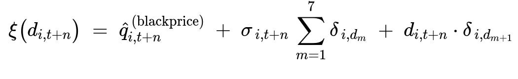
Here:
d_{i,t+n} is the discount in decimal form (0 to 0.7).
hat{q}_{i,t+n}^{(blackprice)} is the predicted demand at zero discount.
sigma_{i,t+n} and delta_{i,d_m} are learned parameters defining how demand scales with discount.
The piecewise linear segments split the 0 to 70% discount range.
Training
Use a loss function that targets accuracy for high-value items more strongly. One option is a weighted square error, weighting each article by a function of its reference (black) price. Freeze near-future decoder in the final phase to focus on far-future predictions. Retrain weekly to cope with new items and shifts in buying patterns.
Production Pipeline
Load data from your warehouse or object store. Preprocess: filter out-of-stock weeks (to avoid misleading sales data), impute partial demand for missing sizes, compute static embeddings, and assemble dynamic covariates. Create training samples by slicing rolling windows. Train on a distributed environment, then push the best model to a prediction service. Generate a demand grid for each article over 15 discount levels and 26 weeks. Hand these predictions to the price optimizer.
Code Example
import torch
import torch.nn as nn

class DemandForecaster(nn.Module):
    def __init__(self, dim_model, num_heads, num_encoder_layers, num_decoder_layers):
        super().__init__()
        self.encoder_layer = nn.TransformerEncoderLayer(d_model=dim_model, nhead=num_heads)
        self.encoder = nn.TransformerEncoder(self.encoder_layer, num_layers=num_encoder_layers)

        self.decoder_layer = nn.TransformerDecoderLayer(d_model=dim_model, nhead=num_heads)
        self.decoder = nn.TransformerDecoder(self.decoder_layer, num_layers=num_decoder_layers)

        # Layers for monotonic demand
        self.mono_price_fc = nn.Linear(dim_model, 8)  # e.g. 7 segments + 1 scale param

    def forward(self, hist_inputs, fut_inputs):
        enc_out = self.encoder(hist_inputs)
        dec_out = self.decoder(fut_inputs, enc_out)
        # Example piece: produce parameters for the monotonic piecewise function
        mono_params = self.mono_price_fc(dec_out)
        return mono_params
Explain every hidden dimension, attention mechanism, learning rate, and batch size. Use dropout for regularization. Insert early-stopping or fine-tuning strategies.
Monitoring
Observe weekly forecasting accuracy on new data. Compare actual sales vs predicted demand. Track aggregated error metrics by product tier, brand, or price segment. Raise alerts if errors exceed thresholds. Adjust model hyperparameters or retrain frequency if performance degrades.
Potential Follow-Up Questions
1) How do you handle new articles with no history?
Use brand and product-category embeddings to tie new items to historically similar articles. Rely on cross-item patterns learned by the global model. For early weeks, guide the estimates with a smaller discount or compare to proven baseline items. Cold starts get refined as real sales data arrives.
2) How do you ensure causal validity when discount changes demand?
Control discount as a direct input. Design a monotonic function so higher discount leads to equal or higher demand. For advanced causal rigor, treat discount as an intervention. One approach is to separate discount assignment from demand signals using domain knowledge or instrumental variables. Another approach is to segment items with stable discount-demand patterns for a tighter focus.
3) How do you handle intermittent demand?
Transform raw sales into a probability-based demand. Impute likely unobserved demand when stock-outs happen. Use a zero-inflated or piecewise approach if demands are extremely sparse. Another approach is to keep the data as is but mask zero-stock intervals, letting the model learn the patterns from other, similar time series in the global model.
4) Why not simpler models like LightGBM or ARIMA?
Global neural networks share parameters across millions of time series. Transformers handle complex interactions and large-scale data efficiently. Tree-based methods may struggle to capture long-range time dependencies or sophisticated cross-temporal patterns. Traditional ARIMA can fail on short, intermittent, or extremely varied time series.
5) How do you decide retraining frequency?
Weekly is often preferred because an online fashion catalog changes fast. Run offline tests to see how forecasts degrade with older models. If the drop is high after two or more weeks, a weekly schedule is safer. Monitor distribution shifts. If major changes happen (new category introductions, new discount policy), trigger earlier retraining.
6) How do you pick the final discount for each article?
A separate price optimizer takes the discount-dependent forecast grid. It chooses the best discount path to maximize profit given inventory and business constraints. This can be done with a mixed-integer or dynamic programming approach. The forecasting system only supplies the discount-demand relationship. The optimizer does the rest.
7) How do you evaluate performance when real data is censored by stock-outs?
Mask or drop periods with no stock. For fairness, measure errors only on weeks with stock available. Keep a separate metric that checks if the forecast direction is consistent with returns from out-of-stock intervals. Ensure the learning pipeline does not blindly trust zero-sales signals.
8) How does the piecewise linear discount function handle large discounts near 70%?
Divide the discount range into fixed-width segments. Let the network learn slope parameters that shift the demand upward more aggressively for deeper discounts. If actual real-world demand saturates at high discount, the learned monotonic function might flatten. Monitor if the model is systematically overestimating or underestimating at extreme discounts.
9) How do you handle big spikes around season transitions or promotions?
Incorporate exogenous signals such as marketing events or season boundaries. Use time-position embeddings to mark key time points, or incorporate a special event covariate. The global model spots repeating surge patterns for big promotions or cyclical transitions (like the start of the holiday season).
10) How do you present final results to management?
Show error metrics that emphasize the monetary impact. Display aggregated Demand Error or Demand Bias weighted by the reference price. Offer a few examples of how discount changes shift demand curves. Demonstrate improved sell-through rate or reduced leftover stock. Combine these outcomes with projected profit improvements from the price optimizer.