
ML Case-study Interview Question: Proactively Predicting Advertiser Churn Using Gradient Boosting Trees

Browse all the ML Case-Studies here.
Case-Study question
You are given a platform where advertisers can run campaigns to reach end-users. The business wants to reduce advertiser churn. Historically, the sales team has reached out only after accounts stop spending. Propose a proactive approach to predict churn probability for currently active advertisers and outline how you would help the sales team prioritize their outreach. Explain the model design, how you define the target variable, how you choose features, and how you validate the impact of your solution.
Detailed Solution
Problem Definition and Rationale
The goal is to predict whether an active advertiser will become inactive within a short time window, so the sales team can intervene before the advertiser actually leaves. This proactive approach is superior to waiting until an account is already lost.
Modeling Approach
A Gradient Boosting Decision Tree (GBDT) solution addresses the tabular data structure. GBDT handles numerical and categorical inputs efficiently. It provides good interpretability through feature importances and cooperates well with Shapley Additive Explanation (SHAP) techniques to explain model outputs.
Defining the Target Variable
An advertiser is considered “active” if they have spent in the last 7 days. If they have no spend in the next 7 days, they are labeled as “churned.” The model predicts if an active advertiser will churn within the next 14 days.
Feature Engineering
The dataset includes approximately 200 features. Each feature is aggregated over multiple time windows. Examples include:
Performance metrics such as impressions, clicks, spend, and conversions.
Usage trends such as weekly or monthly growth in spend or clicks.
Budget and usage pattern data such as campaign creation, edits, or other platform activities.
Advertiser attributes such as account tenure, channel, or industry.
These features capture both historical behaviors and recent shifts. Week-over-week and month-over-month changes illuminate emerging trends in advertiser engagement.
Model Training and Inference
The training set is built by taking “snapshot” data at fixed points in time, labeling whether each advertiser churned or not in the subsequent 14 days. The GBDT model is then trained on these snapshots. After training, each day the system infers churn probabilities for every active advertiser.
Core Probability Computation
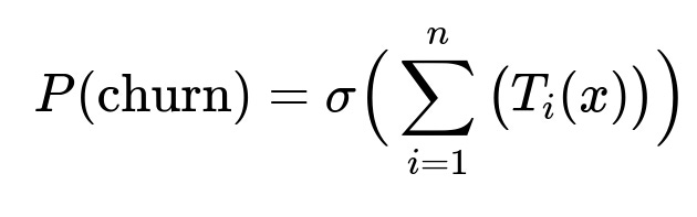
Where:
T_i(x) is the contribution from the i-th decision tree for advertiser data x.
sigma(...) is the logistic function that converts the sum of the tree outputs into a probability.
All inline references to parameters (like n for the number of trees) are in plain text.
Model Explainability
The system uses SHAP to score each feature’s contribution to an advertiser’s churn probability. A positive contribution suggests higher risk. A negative contribution suggests lower risk. The overall probability is the sigmoid of the sum of SHAP values. Sales teams are given top contributing factors, so they know exactly what might be driving the churn risk.
Risk Categorization
Advertisers are split into high, medium, and low-risk categories. Thresholds are established based on desired precision and recall. A high-risk category focuses sales on fewer accounts with greater immediate churn likelihood. A medium-risk category captures the moderately at-risk accounts.
Experimental Evaluation
A controlled experiment compares a treatment group (where account managers see churn risk signals) and a control group (where managers see no churn predictions). Evaluations measure:
Accuracy of predictions (AUC-ROC and AUC-PR).
Churn rate differences between treatment and control.
A 24% churn rate reduction in a pilot segment validates the model’s effectiveness.
Implementation Example in Python
import lightgbm as lgb
import pandas as pd
import numpy as np

# Assume 'data' is a DataFrame with features and 'label' is 0 or 1 for churn
train_data = lgb.Dataset(data, label=label)

params = {
    "objective": "binary",
    "learning_rate": 0.1,
    "num_leaves": 31,
    "metric": ["auc", "binary_logloss"]
}

model = lgb.train(params, train_data, num_boost_round=100)

# For inference
predictions = model.predict(new_data)  # Probability of churn
Short lines of code illustrate how you might train a GBDT model. Additional logic would handle feature engineering, daily batch inference, risk labeling, and handing final results to the sales pipeline.
Follow-Up Question 1: How would you address imbalanced data?
A large portion of active advertisers might not churn in any given period. This imbalance can skew standard metrics.
A practical approach is to use class weighting or oversampling/undersampling methods. Class weighting adjusts the loss function by penalizing misclassifications of the minority class more heavily. Oversampling replicates data from the minority class. Undersampling randomly removes data from the majority class. A mix of these strategies can also be used. Evaluation should rely on metrics like AUC-PR that better reflect performance on rare classes.
Follow-Up Question 2: How would you ensure that new product launches or platform changes do not break the model?
Significant platform changes can cause distribution shifts in features or labels. Monitoring systems that compare past data distributions to current distributions should be in place. If metrics like drift, data coverage, or feature means deviate heavily, retraining the model or updating features is necessary. Retraining on a fixed schedule or more frequently when triggered by drift events maintains model reliability.
Follow-Up Question 3: How would you incorporate sequential models or deep learning architectures?
Sequence-based approaches like a Long Short-Term Memory network or Transformer can learn temporal patterns more directly. Instead of aggregating data over fixed windows, these models learn transitions over time. They can reduce manual feature engineering because they inherently track the temporal relationship. This can improve accuracy, though they demand more data and computational overhead. They also require careful tuning of hyperparameters such as the number of hidden units, dropout rates, and layer depth.
Follow-Up Question 4: How do you handle explainability if you move to a neural network model?
Methods like SHAP can still be used with neural networks, but the explanations might be less intuitive. Layer-wise relevance propagation or integrated gradients can also highlight important inputs. Gradually building trust through robust offline and online tests, combined with partial dependence-style visualizations, helps teams interpret deep learning outputs. Documentation of each feature’s effect is critical for stakeholders.
Follow-Up Question 5: How would you deal with seasonal changes in advertiser behavior?
Seasonality can impact ad spend patterns and conversions. Incorporating seasonal signals (for instance, holiday campaigns) in the feature set helps. Adding time-based interaction variables or a window-based approach captures these shifts. Regular updates to the training dataset ensure the model stays in sync with cyclical changes. If major seasonality shifts occur, specialized models can run during peak times.
Follow-Up Question 6: How do you evaluate the business impact of churn prediction?
The primary metric is reduced churn rate in the treatment group compared to the control group. Secondary metrics include revenue retention or extension of advertiser lifetime value. Statistical significance testing confirms whether observed improvements are not due to chance. Tracking average spend per advertiser over time and correlating improvements with the churn mitigation efforts quantifies the direct business impact.
Follow-Up Question 7: How would you integrate this into a live production pipeline?
A daily or weekly batch job can pull recent activity data, generate features, run the trained model, and output churn probabilities. A subsequent process maps each advertiser to a risk category. The results flow into a user-facing dashboard or a customer relationship management system used by the sales team. Rigorous logging and monitoring ensure stable performance, and data updates confirm that all risk scores stay up-to-date.
Follow-Up Question 8: How do you decide thresholds for high, medium, and low risk?
Sales teams usually prefer high precision for the high-risk group, so they spend time only on accounts that are truly at high risk. Recall is also important. You iterate with the sales team to find thresholds that maintain enough coverage without overwhelming them. Precision-Recall trade-off curves can help. Final thresholds are a business decision informed by model evaluation and resource constraints.
Follow-Up Question 9: What if the advertising budget or conversion metric definitions change?
Changes to budgets or conversion definitions can alter feature distributions and target labels. Detailed documentation of the data pipeline ensures quick adaptation. You might create new features for new metrics and retire old ones that no longer apply. Model versioning helps you track how each change impacts performance. Close collaboration with product and analytics teams keeps data definitions consistent.
Follow-Up Question 10: What if no single model configuration performs well across all advertisers?
Multiple models can be trained to handle specific advertiser segments. For instance, small accounts with lower spend might have different churn indicators than large accounts with higher budgets. Ensemble approaches combine multiple specialized models. The system routes each advertiser to the best model based on attributes like industry, average spend, or region. Clear rules ensure the pipeline automatically selects the correct model.