
ML Case-study Interview Question: Bipartite Graph Neural Networks for Consistent Playlist Song Recommendations.


Browse all the ML Case-Studies here.
Case-Study question
A media streaming platform holds around one million user-created playlists. Each playlist includes multiple songs, each with metadata like artist and album. They want an automated system to extend a partial playlist by adding tracks that fit well with the existing ones. They have large-scale logs of playlists and tracks. They want a machine learning model that, given a playlist, recommends the best songs to keep the style consistent. How would you design and implement such a recommendation engine using graph-based methods?
Provide details on:
Approaches for building a bipartite graph of playlists and tracks.
Graph-based architecture design.
How to split training, validation, and testing edges.
Which loss function to use for ranking and how to handle negative sampling.
How to evaluate top-K recommendations.
What performance metrics to track.
Detailed Solution
Understanding the Data
Data contains one million playlists with track IDs. Each playlist references the tracks it contains. There are also artist and album details, but we focus on a bipartite playlist-track graph. Each playlist node connects to track nodes. An edge exists if the playlist includes that track.
A large dataset can exceed memory limits. A K-core subgraph method selects nodes that exceed a certain degree threshold. This yields a denser subgraph with fewer nodes but richer connectivity. This helps capture strong relationships while reducing training complexity.
Graph Split Strategy
For training, an edge-level split is done (transductive link prediction). We keep all nodes accessible but hide certain edges from the model. The train edges are the message-passing edges for the training stage. Validation edges remain hidden from training but become visible during validation. Test edges remain hidden until the final evaluation.
Model Approach
A playlist node embedding and a track node embedding are learned so that their dot product measures similarity. Tracks with higher dot products are more likely to belong to the playlist. A graph neural network is a strong option because it aggregates neighbor features.
LightGCN, GraphSAGE, and GAT can be tested. LightGCN is lightweight and omits many parameters. GraphSAGE can aggregate neighborhood features in a learnable way. GAT includes attention to weigh certain neighbors more. Layers are stacked to gather multi-hop connectivity.
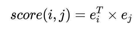
Above is the dot product between playlist embedding e_i and track embedding e_j. Larger values suggest higher similarity.
Each node starts with a learnable embedding. Layers update embeddings by neighbor aggregation. Output embeddings are concatenated or summed across layers to give a final representation.
Loss Function and Negative Sampling
We want a ranking-oriented loss. Bayesian Personalized Ranking (BPR) is common for recommending items. It requires pairs of positive and negative edges for each playlist.
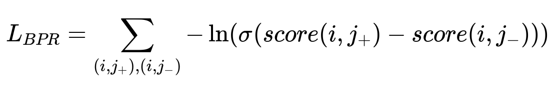
For each playlist i, j_{+} is a known track, j_{-} is a random or hard-chosen negative track. The model learns to rank j_{+} above j_{-}. Hard negatives are chosen from track nodes that the model might already rate highly, pushing it to refine subtle distinctions.
Evaluation
Recall@K is the fraction of true tracks in the top K predictions. Large K ensures we capture enough relevant recommendations. We measure how many correct tracks from the playlist get placed near the top of the model’s ranking.
Example Implementation (Pseudocode)
import torch
import torch.nn.functional as F
from torch_geometric.nn import LGConv, GATConv, SAGEConv

class ExampleGNN(torch.nn.Module):
    def __init__(self, num_nodes, embedding_dim, conv_layer="LGC", num_layers=3):
        super().__init__()
        self.embeddings = torch.nn.Embedding(num_nodes, embedding_dim)
        if conv_layer == "LGC":
            self.convs = torch.nn.ModuleList([LGConv() for _ in range(num_layers)])
        elif conv_layer == "GAT":
            heads = 5
            self.convs = torch.nn.ModuleList([
                GATConv(embedding_dim, embedding_dim, heads=heads, dropout=0.5)
                for _ in range(num_layers)
            ])
            self.post_gat = torch.nn.Linear(heads * embedding_dim, embedding_dim)
        else:
            self.convs = torch.nn.ModuleList([
                SAGEConv(embedding_dim, embedding_dim)
                for _ in range(num_layers)
            ])

    def forward(self, edge_index):
        x = self.embeddings.weight
        x_all = [x]
        for i, conv in enumerate(self.convs):
            x = conv(x, edge_index)
            if isinstance(conv, GATConv):
                x = self.post_gat(x)
            x_all.append(x)
        # Weighted or equal sum
        final_emb = sum(x_all) / len(x_all)
        return final_emb

    def predict_score(self, playlists, tracks, final_emb):
        p_emb = final_emb[playlists]
        t_emb = final_emb[tracks]
        return torch.sum(p_emb * t_emb, dim=1)
The code shows embedding initialization, multiple GNN layers, final embeddings, and a dot product for scoring.
Possible Follow-up Questions
How would you handle scalability when the dataset becomes extremely large?
A sampling or mini-batch approach can be used for message passing. Techniques like GraphSAGE’s neighbor sampling process smaller neighborhood subsets at each layer. Distributed training frameworks can partition the graph. Memory usage can be reduced by training on sub-batches of edges. K-core or other graph pruning ensures relevant nodes remain. Incremental or streaming GNN variants can be used for real-time updates.
Why might you use random negative sampling versus hard negative sampling?
Random sampling is simple and fast. It avoids collisions with positive edges most of the time. Hard sampling focuses on negatives that the model might already score highly, driving finer embedding distinctions. Hard sampling often requires heavier computation to rank many tracks. A hybrid approach can gradually replace random negatives with harder negatives during training.
What if the embeddings collapse into a single dense cluster with little separation?
Over-smoothing occurs when many GNN layers cause embeddings to converge. LightGCN is designed to address this by removing weight matrices and focusing on initial embeddings. Regularization helps maintain variance. You can reduce layer depth or incorporate skip connections. Monitoring cluster variance can signal when over-smoothing occurs.
How do you incorporate additional node features like artist or album metadata?
Construct a heterogeneous graph or a multi-relational setup with separate node types and edges. Graph attention and multi-edge approaches can incorporate those relationships. Alternatively, unify those features into each track node’s initial embedding or add multi-hop edges. If we embed artist and album nodes, we can propagate relevant metadata to track nodes.
What about real-time recommendations when new playlists or tracks appear?
Incremental GNN solutions can update embeddings with partial retraining or neighbor averaging. Streaming GNN frameworks can recalculate embeddings for affected subgraphs. Another strategy is factorizing the node embeddings with a fast update method. This allows newly added nodes to be placed in the embedding space without a full retrain.
How do you ensure the top-K recommended tracks do not violate constraints like explicit content?
Filtering logic can be applied before ranking. Each recommended item can go through a rules-based checker to ensure it meets guidelines. One approach is to create a whitelist or blacklist of tracks. The final top-K are chosen from permissible candidates only.
How would you productionize this system at scale?
A pipeline would handle data ingestion, graph construction, and incremental updates. A stored model generates embeddings or uses a real-time serving layer for quick inference. Edge-based sampling can run daily or hourly, depending on volume. Automated evaluation monitors recall metrics on fresh playlists. Parallelization or GPU clusters handle large-scale inference.