
ML Case-study Interview Question: Gradient Boosting for Precise Delivery Service Time Estimation and Route Optimization.

Browse all the ML Case-Studies here.
Case-Study question
You are given data on delivery stop events where each stop’s “service time” is the time spent parking, unloading, and delivering items. The service time can be about half of a driver’s workday. You also have the route structure, with around 30 stops per route. The route planner uses service time and driving time estimates to schedule deliveries. Historically, a simple rule-based model predicted service time. It worked acceptably on an aggregate level but was inaccurate at individual stop level, especially in dense urban areas versus rural areas. You want to build a machine learning model that more accurately predicts service time for each stop, then integrate this into a route planner to reduce overall lateness and improve on-time rates. How would you design, train, and deploy this model? How would you handle messy data, drift, and real-world test strategies?
Proposed solution
Data collection
Geofence-based tracking is set up to measure how long a driver spends for each stop. The system logs the time a driver enters a geofenced region and the time they leave. Each record becomes a labeled data point for supervised learning. Data might be noisy or incomplete, so careful filtering is crucial. Outliers arise from drivers pausing between stops, failing to scan deliveries immediately, or entering the same geofenced region multiple times.
Feature engineering
Order size, weight, number of items, and package count affect unloading time. Parking challenges are different in dense areas than in less populated areas, so location-based features can help. Building characteristics such as floor level or elevator availability can also matter. For new or infrequent addresses, robust default assumptions are needed until enough data is collected.
Model architecture
A gradient boosting model such as LightGBM learns complex interactions among numeric and categorical features. A possible training objective is minimizing Mean Absolute Error (MAE). The core loss function used to measure model performance can be represented as
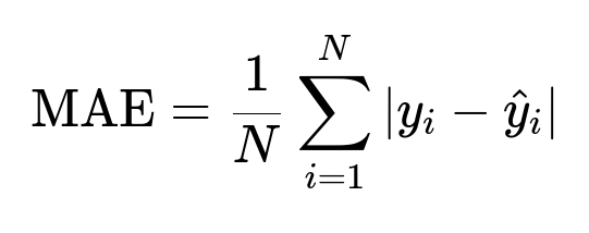
y_i is the actual service time of the i-th data point. hat{y}_i is the predicted service time of the i-th data point. N is the total number of data points in the training set.
Bayesian optimization techniques like optuna can be used for hyperparameter tuning to find the best learning rate, depth, and other parameters. The final model outputs a numeric service time prediction for each stop.
Real-world validation
The model is tested in a representative region first. Only that region uses the new ML-based predictions, while the rest still uses the older rule-based approach. This allows direct comparison of performance metrics such as MAE and scheduling delays. Any anomalies in the early test region can be investigated without disrupting the entire system.
Route planner integration
The route planner now receives more precise service time estimates for each stop. It calculates the total route duration by summing service times for all stops plus the driving times between them. If the model still has systematic biases, the route planner might inadvertently overshoot or underestimate total time. The final metric is the distribution of lateness across all stops. The goal is to shrink the variation in arrival times around zero delay.
Results and improvement areas
Even with more accurate predictions, overall lateness improvement might be modest if inaccuracies cancel out when aggregating 30 stops on a route. Urban stops might take longer than planned, and rural stops might be faster. The net effect can appear acceptable in total route duration. Further work includes filtering faulty training data more aggressively, adding weather data for snow conditions, and implementing a retraining or active learning pipeline so the model adapts as driver skills change or new markets are opened.
What if the model doesn’t improve lateness enough?
Suboptimal route planner logic might be overshadowing the benefits of precise sub-component forecasts. Route planning might need refinements to fully leverage the improved service time estimates. The system can also incorporate dynamic adjustments if stops run significantly ahead or behind schedule, balancing future deliveries more effectively.
Follow-up question 1
What alternative loss functions or evaluation metrics would you consider, and why?
Answer Some practitioners prefer Mean Squared Error (MSE) to punish larger mistakes more heavily, which can be valuable if large errors are most costly. Others might use quantile loss if they care about worst-case scenarios. A high Quantile (like 90th percentile) can be valuable for operational planning because a few extreme delays might seriously impact performance. Another approach is Weighted MAE if certain deliveries or time windows are more critical.
Follow-up question 2
How would you clean the training data to remove inconsistent geofence measurements?
Answer Records can be filtered by feasible time thresholds. Extremely short or unreasonably long durations might indicate sensor errors or driver behavior anomalies. Logging data should be cross-referenced with scanning events and route logs. Stops with missing or contradictory time stamps are removed. A practical strategy is to define upper and lower cutoffs based on historical percentiles to discard outliers. Another technique is building an anomaly detection module using an unsupervised model to flag suspicious events.
Follow-up question 3
How would you handle new locations without much historical data?
Answer A fallback approach might use averages from similar neighborhoods or rely on the rule-based model for a period. Over time, data from the new location is accumulated, and the model updates. One option is using hierarchical location-based features, where unknown addresses inherit estimates from broader geographical clusters until local data becomes sufficient. An exploration bonus can be added to new addresses, allowing the system to adapt quickly once real data arrives.
Follow-up question 4
Explain how you would incorporate weather data into your training pipeline.
Answer A weather feature can be added to each row in the training set by matching timestamp and location with a weather database. Temperature, precipitation, or snowfall might prolong unloading times. The model can learn these correlations if they are consistent. A preprocessing step merges historical weather records with the service time logs, labeling each training event with weather conditions. For real-time predictions, the model is fed current or forecasted weather data to predict more accurately on days with harsh weather.
Follow-up question 5
How could you manage model drift or distribution shifts when expanding to new markets?
Answer A continuous retraining loop is set up, ingesting recent data in short intervals. If the distribution changes abruptly, a reference set of performance metrics can detect degraded accuracy. The system automatically triggers partial retraining or hyperparameter optimization. Transfer learning or domain adaptation can be used if the new market significantly differs in geography or traffic patterns. A track of “exploration” in early deliveries of new markets can refine estimates quickly by deliberately capturing more varied data points.
Follow-up question 6
What if your model systematically underestimates certain delivery contexts?
Answer Model explanation tools like SHAP can detect if certain features (like a specific building type or neighborhood) are consistently mispredicted. Analysts can investigate whether those stops require extra features (e.g., does the neighborhood have limited parking?). Corrective terms can be added. Weighted training or separate specialized sub-models can also remedy systematic underestimation.
Follow-up question 7
Could a different model type or ensemble approach outperform LightGBM?
Answer An ensemble combining gradient boosting with neural networks or random forests might improve marginally, especially if the data is high-dimensional. Neural networks can capture interactions if sufficient data is available, but training is more complex. Gradient boosting is often a strong baseline for tabular data. The best approach is to experiment with multiple architectures and compare validation performance. Deploying the simplest model that meets performance goals is generally preferable for reliability and easier maintenance.