
ML Case-study Interview Question: Contextual Bandits for Dynamic Selection of Personalized Item Ranking Methods


Browse all the ML Case-Studies here.
Case-Study question
A tech firm introduced multiple ways of ranking recommended items. Each ranking method prioritized a different combination of objectives such as personalized relevance, popularity, price, and availability. They randomly assigned users to each method to collect training data. The goal is to build a Contextual Bandit model that, for every new user and context, selects the ranking approach that maximizes cart additions per search while maintaining healthy revenue. How would you design such a solution?
Detailed Solution
Use a Contextual Bandit (CB) model that treats each ranking method as a discrete action. Include key user attributes and query features in the context vector. Train on logged data where each action was randomly selected, and measure the reward as items added to cart or a similar engagement metric.
Preprocess your data into (context, action, reward) tuples. Build a model that, given the context, predicts the expected reward for each action. Some standard approaches:
XGBoost with an Action Feature Treat the action (ranking method) as a categorical feature. Train on logged data to predict reward. At inference, create one copy of the context per possible action, set that action feature accordingly, and pick the action with the highest predicted reward.
Neural Network with Multi-Output Use a network with an output node for each action. Backpropagate the error only through the node corresponding to the chosen action. Then choose the action with the highest output at inference.
X-learner Train first-level models to predict reward for each action group. Then train second-level models to predict each action’s incremental lift relative to a baseline. Pick the action with the largest predicted lift in new contexts.
Below is an example formula for a multi-objective ranking score that might be one of the candidate actions the Contextual Bandit chooses:

Here, w_rel, w_pop, w_price, and w_avail are relative weights for each objective.
When evaluating the policy offline, use inverse propensity sampling (IPS) or doubly robust (DR) estimators. An IPS estimator for a new policy p_new given old logging policy p_0 is often expressed as:
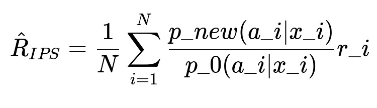
N is the total number of logged events. x_i is the context, a_i is the action taken, r_i is the observed reward. p_new(a_i|x_i) is the new policy’s probability of that action for context x_i, and p_0(a_i|x_i) is the old policy’s probability. This ratio weighs each observed reward by how often the new policy would select that same action compared to the old policy.
Technologies and Rationale
Combine a CB model with discrete actions for each ranking formula. Train on a randomized dataset collected by assigning each user to a random ranking approach. Use offline evaluation to filter out poor policies before deployment. If continuous parameter tuning is needed (e.g., you want to search over weighting vectors instead of fixed discrete actions), consider policy gradient methods or an RL approach supporting continuous action spaces.
If you require a library for training, frameworks like RLlib can handle offline CB or RL workflows. Prepare data in a format the framework expects (e.g., JSON lines of (state, action, reward)). Use standard configurations or custom hyperparameters to train a DQN or any other suitable method. Periodically compute IPS or DR metrics to gauge policy performance. Deploy the best-performing checkpoint to production for final A/B testing.
Implementation Example
A basic Python snippet for offline training with RLlib’s DQN could look like this:
from ray import tune
from ray.rllib.algorithms.dqn.dqn import DQNConfig

config = (
    DQNConfig()
    .offline(input_config={"format": "json", "paths": ["path/to/logged_data.json"]})
    .training(gamma=0, model={"hidden_dim": 64})
)

tuner = tune.Tuner(
    "DQN",
    param_space=config
)

results = tuner.fit()
Offline metrics like IPS or DR guide you to the best epoch. Then serve the resulting policy.
Under-the-Hood Reasoning
A multi-armed bandit treats actions without user-specific context, learning an overall best action. A contextual bandit extends this by conditioning on user features or query attributes. This improves personalization for diverse user intentions. For large action spaces (many ranking methods or embedded vectors), it is critical to reduce complexity by defining a manageable set of discrete actions or by using an embedding approach with advanced off-policy evaluation techniques.
How would you handle high-dimensional user features or item embeddings?
Use feature hashing or dimensionality reduction. If item embeddings are large, train a CB that outputs preference vectors over embedding clusters. Or approximate the reward function with a model that infers how features map to reward, then pick the highest reward–generating subspace.
How do you ensure adequate exploration in data collection?
Randomly assign ranking methods in your experiment, ensuring every method is tried enough. Control randomization probabilities so the more promising methods get somewhat higher probability. This trades off between gathering data for all actions and exploiting known good actions.
If you wanted to optimize for multiple metrics (e.g., cart additions and revenue), how would you design the reward?
Combine them into a scalar. For instance, assign a suitable weight to each component. If cart additions per search is crucial but revenue per search matters, define a reward = alpha * cart_adds + (1 - alpha) * revenue. Calibrate alpha after experimentation and possibly treat that alpha as part of the action space.
Why might you choose an X-learner over a simpler supervised approach?
X-learner directly models incremental lift relative to a baseline action. This helps measure how much better or worse a new approach is compared to the current production. It can reduce bias when data is imbalanced or when one action is more frequent, since each specialized model focuses on incremental effects rather than fitting a single global function.
How would you approach latency constraints in large-scale production?
Use lightweight models like gradient-boosted trees or small neural networks. Precompute partial features or scores if possible. For big neural nets, distill them into smaller networks or use model compression. Evaluate the cost of recomputing the reward predictions for every action. If the action set is small (e.g., 5–10 ranking formulas), the latency overhead remains acceptable.