ML Case-study Interview Question: Adaptive Anomaly Detection for Multi-Dimensional Time Series Using Seasonality and Feedback.

Browse all the ML Case-Studies here.

Case-Study question

You are tasked with designing and deploying a system that detects anomalous behavior in multi-dimensional time series data for an online marketplace. The data includes metrics such as transactions, payments, performance indicators, and user interactions, each having multiple attributes (e.g., region, product category, payment type). Many issues are high-frequency and are quickly detected by standard monitoring tools, but a large number of lower-frequency issues or small-segment issues slip under the radar. These low-volume anomalies accumulate into user dissatisfaction and potential revenue loss over time. The requirement is to automatically identify, rank, and alert on these anomalies, and then incorporate user feedback to refine detection over time. How would you build and implement this system?

Detailed Solution

Use a modular pipeline with these main components:

Onboarding and Metric Configuration. Allow metrics to be onboarded easily via a user interface or API. Store each metric’s configuration, define the dimensions and the granularity.

Multi-Dimensional Metric Cube. Extract all valid dimensional combinations and generate small slices of the data for targeted detection. This transforms the raw data into segments such as (region=XYZ, product=ABC, currency_code=QQQ) for fine-grained monitoring.

Data Profiling. Evaluate the incoming data quality. Identify missing values, outliers, or potential data distribution shifts before feeding to model selection steps.

Seasonality Detection. For each slice, detect if it has cyclical behavior. Seasonal slices follow decomposition-based methods; non-seasonal slices apply simpler statistical tests. Track patterns that repeat daily, weekly, or monthly.

Model Selection and Execution. For seasonal data, prefer decomposition-based methods or models like STL (Seasonal and Trend decomposition using Loess) or open source forecasting libraries that handle cyclicality. For non-seasonal data, use simpler statistical methods (e.g., z-score, interquartile range, standard deviation). Profile each slice in real-time, select a suitable model, and generate anomaly signals.

Rules Engine. Combine signals from different models, attach business rules (generic or exception-based), and score anomalies. Implement significance scoring to rank anomalies based on factors like the size of deviation from the mean and the segment’s contribution to overall traffic.

Publishing and Notification. Publish anomalies that pass relevance thresholds. Send alerts through email or popular chat tools with details on the time series slice, severity, and direct links to a dashboard or logs. This allows quick investigation.

Feedback Loop. Collect user feedback to label anomalies as true positive or false positive. Store these labels and feed them to a learning component that can generate new exception rules. Example: a city with negligible traffic might trigger a disproportionate number of low-value anomalies, so the system learns to suppress or re-rank them.

Scaling and Performance. Use a distributed computing framework for large-scale data (millions of series). This reduces computational overhead. Transition from heavy data manipulation libraries to more efficient frameworks to improve run times.

Continuous Improvement. Continuously measure precision, recall, and F1 score. Retrain or switch models if performance degrades. Iterate on the seasonality detector and the significance scoring to reduce false alarms and missed anomalies.

Example Python snippet for a seasonal method (STL) on one data slice:

import pandas as pd
from statsmodels.tsa.seasonal import STL
import numpy as np

# Suppose 'df' has a DateTime index and a 'metric_value' column
df = df.sort_index()

# Apply STL for decomposition
stl = STL(df['metric_value'], period=7)  # weekly seasonality example
res = stl.fit()

# Anomaly detection using residual
threshold = 3.0 * np.std(res.resid)
df['resid'] = res.resid
df['anomaly_flag'] = df['resid'].apply(lambda x: 1 if abs(x) > threshold else 0)

This snippet shows how a single slice’s anomalies might be flagged, which then get combined with signals from other models in the pipeline.

F1 Score Formula

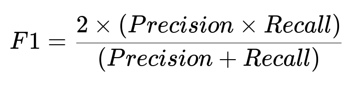
Precision is the fraction of detected anomalies that are truly anomalies. Recall is the fraction of all true anomalies correctly identified. Higher F1 implies a balanced performance of detecting genuine anomalies while minimizing false alerts.

Follow-up Question 1: How do you handle seasonality detection for multiple seasonal periods (e.g., daily and weekly cycles) in high-frequency data?

Multiple decomposition models can be applied when a single seasonal period is insufficient. One approach is to run a repeated decomposition across daily and weekly frequencies. Another method is to extend the STL approach to support multiple seasonalities or to use a specialized library that handles multiple cycles. A practical example is modeling one period at a time, removing it, and then modeling another. Compare the residuals after each stage. Track root mean square error (RMSE) and mean absolute percentage error (MAPE) to see if removing those seasonalities improved overall fit. If the data slice has strong multiple peaks, a multi-seasonal decomposition reduces false positives caused by unaccounted-for cycles.

Follow-up Question 2: How do you reduce false positives for low-traffic segments?

Use a classification-based approach or user feedback signals that distinguish whether fluctuations in low-traffic segments are business-actionable. One practical solution is tiering segments based on volume. Top-tier segments produce high-impact anomalies, so keep them at standard thresholds. Bottom-tier segments produce many small fluctuations, so raise thresholds or group them until they reach enough volume to be meaningful. Another option is to incorporate user-defined exception rules that explicitly ignore or re-rank anomalies from those low-volume segments. Whenever users label an anomaly as not actionable, store it in a feedback database to retrain or update these rules automatically.

Follow-up Question 3: How do you incorporate user feedback to refine anomaly detection?

Maintain a labeled repository of anomalies. Whenever users mark anomalies as “false” or “true,” store the context (metric name, dimension, date-time range, detection method used). A feedback processing module scans these labels and looks for consistent patterns. Example: a city named “CityX” that always triggers “false” anomalies at certain hours. Generate an exception rule to ignore or re-rank anomalies from that context. Retrain or fine-tune model hyperparameters. Continuously track precision and recall on new data to confirm that your changes improve system performance without under-detecting real issues.

Follow-up Question 4: How do you handle near real-time anomaly detection?

Adopt a streaming pipeline. For each incoming data batch or event, apply a lightweight model (e.g., a streaming statistical approach or a pre-trained decomposition model) to estimate the expected value and compare with the actual. Keep the more complex seasonal detection or retraining tasks in an offline job. Maintain a small in-memory buffer of recent data points. Make near real-time alerts actionable by providing a quick analysis (e.g., dimension breakdown) so on-call teams can respond. If advanced forecasting models are used, store updated seasonal components offline so the online layer can quickly reference them without heavy computations during streaming.

Follow-up Question 5: How do you ensure the system is performant at scale?

Distribute computations across a cluster using tools optimized for large-scale data. Replace memory-intensive data manipulation in single-node libraries with more distributed frameworks for tasks like data preprocessing, outlier scoring, and significance ranking. Profile each pipeline stage to measure runtime. Optimize data partitioning to prevent large data shuffles or re-partitions. Cache intermediate results where possible, and push only aggregated anomalies downstream. This approach enables you to process millions of time series data points daily without bottlenecks or timeouts.

---