
ML Case-study Interview Question: Neural Network Revenue Prediction for Dynamic Ad Request Filtering


Browse all the ML Case-Studies here.
Case-Study question
A large social platform faces huge incoming ad requests from two sources: (1) their own platform, and (2) third-party apps that connect to external advertisers. The platform’s ad server can return relevant ad candidates for many of these requests, but it needs to drop a significant portion to save resources and focus on higher-value requests. Initially they used a simple heuristic: track how many times a specific (device, app) pair produced zero impressions, then drop future requests from that pair if it crosses a threshold. This saved computation but removed some potentially valuable requests. They want a more robust approach that automatically adapts to incoming request patterns. They built a lightweight feedforward neural network model to predict each request’s expected revenue, then used a dynamically adjusted threshold to filter low-scoring requests. Their new system reduced request load by more than half, raised total revenue, and improved system metrics. Propose a solution strategy, including how you would handle feature engineering, model architecture, training loop, inference pipelines, and system performance monitoring.
Detailed solution
Features can include user-level signals such as device IDs or user IDs, contextual features like app category, geo-locations, or timestamps, and historical interaction patterns such as how many times a similar request led to an impression. A minimal set might replicate the heuristic’s features (device ID, app category, and recent success frequency), but adding more signals can improve accuracy.
A simple feedforward neural network can suffice. One hidden layer, or two at most, keeps the model small. For each incoming request, feed the feature vector x into the network to get a predicted revenue y_hat. A typical feedforward network performs weighted transformations of x through hidden layers and outputs a final scalar.
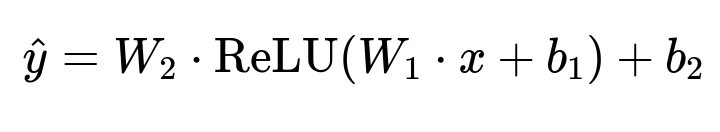
Where x is the input feature vector, W_1 and W_2 are weight matrices for the hidden and output layers, b_1 and b_2 are bias terms, and ReLU is the chosen activation function.
Continuous training updates the parameters on recent data. The system calculates loss by comparing predicted revenue with actual revenue. This might be total money earned from that request or a proxy metric (clicks or conversions). Each hour, a newly trained model is produced. A “score histogram” of past model predictions determines a cutoff for what fraction of requests to allow. If we want to allow 50% of requests, pick the predicted revenue threshold at the 50th percentile in that histogram.
Implementation requires a training pipeline that logs request features and true outcomes in near-real-time. A job processes recent data to train the model. In production, a stateless inference service loads the latest model, scores each request, and decides pass/fail based on the updated cutoff.
System performance hinges on monitoring key metrics: total revenue, request load, latency, error rates, and success rates for the top traffic segments. If the model is too strict, revenue might drop, or user metrics might degrade. If the threshold is too low, the system might process too many low-value requests. Automated dashboards track these metrics, plus model prediction quality over time.
What if the heuristic threshold no longer adapts to changing patterns?
The heuristic must be manually tuned. A small shift in user or advertiser behavior might render the old threshold useless. The ML approach dynamically learns patterns from new data and calibrates the cutoff via the real-time histogram. This self-adjustment keeps performance stable.
How would you handle data freshness?
Regularly retrain on up-to-date logs. For an hourly or daily cadence, gather the latest requests, compute real revenue or success metrics, then update weights. A rolling window approach (for example, last 24 hours) ensures the model always reflects current behavior. If distribution shifts are faster, reduce the training window or increase training frequency.
Why is a small model sufficient?
A single or double-layer network can capture basic interactions among request features. Extensive hyperparameter optimization might give diminishing returns relative to the costs of bigger models. Smaller models keep inference latency low, which is crucial at high request volume.
How to handle incomplete data or new users and apps?
Impute missing features with defaults or special embeddings. Use fallback logic when you see a never-before-seen feature combination. For example, treat new (device, app) pairs as moderate-value until enough data accumulates. The model learns patterns from similar known features and generalizes.
How to scale further if the traffic volume doubles?
Scale horizontally by deploying more instances of the scoring service. Ensure the feature retrieval pipeline is efficient. Consider a more compressed model or faster run-time libraries. Keep logging and retraining pipelines robust enough to handle higher throughput. Leverage distributed systems for data collection and training.
What if you need more advanced deep learning?
Experiment with deeper networks or specialized layers (embedding layers for categorical features, gating mechanisms for user contexts). Evaluate cost-benefit tradeoffs. If a small feedforward net already performs well, more complexity might not justify the increased overhead.
How to guarantee no unintended bias?
Monitor feature usage to avoid problematic or sensitive data. Track metrics across demographic segments. If certain segments are under-served, revisit the training process or add constraints. Use fairness metrics as additional objectives. Regularly audit predictions for bias or unexpected patterns.