
ML Case-study Interview Question: Predicting Food Delivery ETA with XGBoost and Real-Time Features

Browse all the ML Case-Studies here.
Case-Study question
You are asked to build a system for a large-scale food delivery platform that must predict the time of food arrival to customers. The platform has millions of users and thousands of restaurant partners. Customers often abandon their carts if the displayed delivery time seems too long, and they also lose trust in the platform if the actual delivery time exceeds the estimate. The task is to propose an end-to-end data science solution to generate delivery time predictions, incorporate real-time order-level features, and ensure these predictions remain accurate over time. How would you design, implement, and maintain such a system?
Detailed In-Depth Solution
This system requires modeling the total time between order creation and food arrival as a numerical variable. It can be treated as a regression problem using historical orders as training data.
Model Approach
The main target is how many minutes (or seconds) it takes for food to arrive. It can be predicted as a single wholesome value (total time) or as the sum of sub-components:
Time from order acceptance to the driver reaching the restaurant (T1).
Time for the driver to pick up the food at the restaurant (T2).
Time from pickup to final delivery (T3).
Splitting into components gives more control over each phase. Each sub-component has different influential features, such as merchant trends, time of day, order value, and distance.
Key Metrics
Performance can be measured with common regression metrics. Three core metrics:
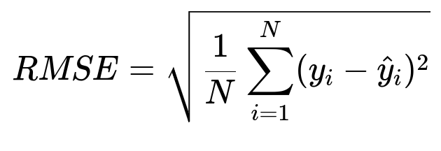
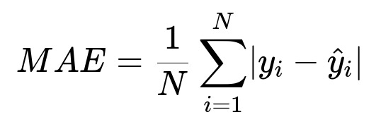
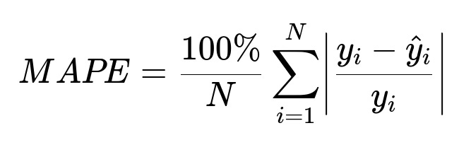
Where y_i is the actual time, and hat{y}_i is the predicted time for the ith order. RMSE penalizes large errors more, MAE treats all errors equally, and MAPE shows the percent deviation from the actual value.
Real-world monitoring also includes:
Compliance: Ensuring the predicted time does not fall below the actual time too often (under-prediction).
Conversion: Observing if a higher predicted time reduces the chance of customers completing the order.
Model Training
A gradient boosting approach (like XGBoost) is effective. Historical order data is collected for a few weeks. Features are aggregated by merchant, hour of day, distance category, order items, and average times for each phase (T1, T2, T3). Additional real-time features are needed at checkout (order value, live traffic distance, number of items, etc.).
A wholesome model can directly predict total arrival time. A split approach has three separate models for T1, T2, T3, then sums them up. This often yields better overall performance.
Implementation Details
Some sub-components do not need personalization for each user (e.g., T1 or T2 in discovery pages) because many features are aggregated by merchant and hour. These can be batched. If more granular real-time features (distance, order value) become available at checkout, an online prediction service can fetch the relevant features from a feature store and call the model in real-time.
In practice:
A batch process runs hourly or daily for T1, T2, T3 at the merchant level or distance-based level.
The results are cached in a fast data store.
For checkout predictions, a real-time service queries features, then calls an online model to infer T1, T2, T3.
The final ETA is the sum of T1 + T2 + T3 or the wholesome model output.
Below is a minimal Python code snippet illustrating an XGBoost training loop:
import xgboost as xgb
import pandas as pd

# Suppose df has columns: features..., and 'target' is the total time or a sub-component (T1, T2, or T3).
train_data = xgb.DMatrix(data=df[feature_cols], label=df['target'])

params = {
    "objective": "reg:squarederror",
    "eta": 0.1,
    "max_depth": 6,
    "subsample": 0.8
}

model = xgb.train(params, train_data, num_boost_round=100)

# Then save model for batch or online use
model.save_model("delivery_eta_model.json")
Future Extensions
Retraining frequently (daily or weekly) keeps the model updated with evolving merchant behavior and traffic patterns. Additional data sources, such as queue length at restaurants or driver acceptance likelihood, can further refine predictions.
How would you handle missing or sparse historical data for new merchants?
Sparse data often appears when a new merchant or location joins the platform. A fallback approach uses similarity-based features (e.g., average times of nearby merchants, or overall city averages) for bootstrapping. Over time, more direct data from the merchant accumulates, and the model shifts to merchant-specific features.
How do you ensure real-time feature availability?
A feature store is essential. It stores precomputed aggregations and can serve them at low latency. For dynamic features (e.g., driver distance to merchant), an orchestration layer fetches those from a live service. If a feature is temporarily unavailable, a default or fallback logic is used.
How do you avoid under-predicting too often?
Loss functions and post-processing can be adjusted. Adding a small buffer (safety margin) to predictions reduces under-prediction. Alternatively, a quantile regression approach can be tried to bias predictions above the median or some percentile of error.
How would you monitor model drift?
Statistics on error distributions are tracked. If the mean absolute error spikes or the compliance metric drops, it signals potential drift. Retraining or adjusting features might be triggered if certain merchants or locations show persistent mispredictions.
How do you scale it to millions of orders each day?
A mix of hourly or daily batch predictions for broad-level features and real-time inference for critical personalization is used. Batch jobs run on a large compute cluster and update aggregated features. The online prediction service is autoscaled to handle peak traffic. Caching results for popular merchant-distance pairs helps reduce repeated computation.
How do you handle outliers or extreme durations?
Some orders can suffer from driver unavailability or restaurant delays. These extremes can skew the model. Clipping or capping target times at a certain percentile or employing robust loss functions (like Huber loss) makes the model less sensitive to large outliers.
How do you measure the business impact?
A/B testing is done. The new model is compared to a baseline approach on a subset of users. Key metrics:
Conversion improvements.
Reduction in average error.
Increase in repeat orders or user satisfaction.
These metrics confirm if the updated system effectively balances accurate times and user trust.