ML Case-study Interview Question: Architecting a Scalable Forecasting System using XGBoost and Exogenous Features

Browse all the ML Case-Studies here.

Case-Study question

You are working at a large technology company that supports multiple use-cases under a single platform. Different teams require accurate daily forecasts for resource allocation, strategic planning, and operational decisions. Many teams rely on basic spreadsheet solutions or simple time series models. Some more advanced teams use ARIMA or Exponential Smoothing (ETS), but they do not incorporate external variables. A senior analyst prototyped an end-to-end forecasting tool that combines holiday indicators, calendar signatures, and lagging features in XGBoost, giving significantly improved forecasts compared to other methods. They then built a user interface so non-technical stakeholders could generate forecasts in just a few clicks. Your task is to propose how to architect this forecasting system from the ground up, outline a methodology to handle exogenous factors (e.g., shifting holiday periods or spending data), and describe how you would evaluate, deploy, and maintain this tool for various teams.

Detailed Solution

Overview of the System

A robust solution integrates feature engineering, model training, and prediction in a pipeline accessible to non-technical users. It automates hyperparameter tuning, handles time series cross-validation, and provides a quick interface for scenario-based forecasts. It must incorporate external data such as holiday flags, marketing spend, or other relevant signals.

Choice of Algorithms

ARIMA and ETS are popular classical methods. Multiple Linear Regression (MLR) can incorporate external variables, but it may underfit complex relationships. XGBoost has shown superior performance by capturing non-linear relationships and integrating external features. Comparative experiments using real datasets indicated that XGBoost with holiday information yields about 10% lower median mean absolute percentage error (MAPE) than ARIMA or ETS.

Main Metric

MAPE is a common measure of forecast accuracy. The lower the MAPE, the closer the predictions are to the actuals.

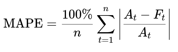
Here, A_t is the actual value at time t, F_t is the forecast at time t, and n is the total number of forecasted points. This quantifies percentage error relative to the scale of the actual data.

Time Series Cross-Validation (TS CV)

Time-aware cross-validation ensures the model never trains on future data when predicting earlier points. This is done by incrementally expanding the training window and preserving the chronological order in each fold. Normal random cross-validation often overestimates performance for time-series tasks because it allows leakage from future data. TS CV reduces such bias and provides a more realistic estimate of errors.

Feature Engineering

Holiday flags capture spikes and dips during festivals or seasonal events. Lagged values of the target help XGBoost learn autocorrelations. Additional calendar signatures (day-of-week, week-of-year, month, year) add seasonality signals. Spending and other exogenous inputs capture relevant external impacts. The model benefits from these features when training on historical data.

Tool Architecture

A backend service triggers data extraction and feature generation for each forecast request. It then runs automated hyperparameter tuning (e.g., grid search or Bayesian optimization) on XGBoost, using TS CV to pick the best model configuration. It stores the trained model and outputs forecasted values for the requested horizon. An interface allows any business user to generate forecasts for multiple units, such as different cities or product lines, in a single run. Users can modify certain inputs (like budgets or holiday assumptions) to see alternative forecast scenarios.

Performance Interpretation and Explainability

The system ranks feature importance to reveal major influences on the forecast (e.g., holiday data, lagged values). This helps business stakeholders understand how changes in one variable affect the target. The TS CV metrics give a window into possible uncertainty. If the forecast horizon is far beyond the range of the training data, XGBoost may struggle to extrapolate. Future versions can incorporate stacking with other models and produce aggregated forecasts at different levels of granularity.

Practical Implementation

Use a pipeline approach in Python. For example:

import pandas as pd
import xgboost as xgb
from sklearn.model_selection import ParameterGrid
from sklearn.metrics import mean_absolute_percentage_error

# Example data loading and feature engineering
df = pd.read_csv("data.csv")
df["lag_1"] = df["target"].shift(1)
df["is_holiday"] = (df["date"].isin(holiday_dates)).astype(int)
# Add more features as needed

# Time series cross-validation function
def time_series_cv(data, param_grid, folds=4):
    best_mapes = []
    best_params = None
    for params in ParameterGrid(param_grid):
        mapes = []
        for fold in range(folds):
            # Split data into train/validation respecting time
            # Train model
            xgb_model = xgb.XGBRegressor(**params)
            # Evaluate
            # Collect MAPE
            mapes.append(current_fold_mape)
        avg_mape = sum(mapes) / folds
        if not best_params or avg_mape < min(best_mapes, default=1e9):
            best_mapes.append(avg_mape)
            best_params = params
    return best_params

# Hyperparameter tuning
param_grid = {
    "n_estimators": [100, 200],
    "learning_rate": [0.01, 0.1],
    "max_depth": [3, 5]
}
best_params = time_series_cv(df, param_grid)
# Retrain final model on entire dataset with best_params and predict

Models and results can be stored in a database. A front-end or notebook interface can access them. This workflow ensures consistent forecasting across teams without deep knowledge of advanced time-series methods.

Potential Follow-up Questions

How would you extend the solution to handle multiple time granularities and hierarchical forecasts?

A hierarchical scenario involves forecasts at various levels (e.g., city, region, country) and time resolutions (daily, weekly). Summing up daily city-level forecasts might not match the weekly aggregate. A reconciliation step like bottom-up, top-down, or middle-out solves these discrepancies. A shared data pipeline processes base features. A hierarchical model can use advanced approaches like grouped time series training or prediction reconciliation. This ensures consistent forecasts across all aggregation levels. One strategy is to train a single model with a group identifier, then predict per group and reconcile predictions using post-processing. Another approach is to train separate models for each level and align them via an optimization procedure so the sum of lower-level predictions equals the higher-level forecast. Teams typically prioritize a top-down approach when the upper-level forecasts are more reliable or have better data. Bottom-up is preferred when granular-level data is more accurate or stable.

How would you maintain model performance over time and handle concept drift?

Drift occurs when relationships in the data shift, possibly due to new promotional campaigns, user behavior changes, or external market dynamics. Monitoring involves tracking MAPE or other metrics on recent forecasts. Anomalies in error patterns suggest retraining or feature updates. A weekly or monthly retraining schedule is common if enough new data is available. If drift is severe, more frequent training is required. In production, a rolling retrain approach is used. You can automate alerts when forecast errors exceed predefined thresholds. If the model starts to degrade significantly, investigate new features or revisit hyperparameters. Maintaining a versioned history of models and data ensures reproducibility. Retraining also includes verifying holiday definitions, adding new external signals, or adjusting seasonality features. Feature drift can be addressed by refining existing transformations or adding relevant real-time signals. Tests in a staging environment confirm stability before pushing the updated model to production.

What if your time series has intermittent zero values or is extremely sparse?

Sparse data is common in some niche products or smaller markets. XGBoost may still handle it, but certain lags become zero or undefined. One approach is aggregating the data to weekly or monthly intervals to smooth out zeroes. Another approach is building a separate classification model that predicts the probability of non-zero values, then a regression model for magnitude. This two-stage method helps if your data is zero-inflated. You can also explore specialized models like Croston’s method or Holt-Winters for intermittent demand, though these methods can be limited in handling external features. Testing multiple strategies is important. If you do a two-stage approach, the classification part might incorporate external signals that often trigger demand. The regression then refines the quantity given that demand is non-zero.

How would you incorporate scenario-based forecasting?

The tool allows users to adjust certain external variables (holiday schedules, marketing budgets, or pricing changes) and generate new forecasts. When the system fetches features for the future horizon, it sets them according to each scenario. The trained model then outputs the predicted target. This helps stakeholders weigh possible outcomes under different business strategies. For instance, a marketing manager might want to see how a budget increase of 20% affects next quarter’s sales. The system simply uses that 20% boost in the feature column for each future date, re-runs the model inference, and returns the forecast. If seasonality or holiday timing also shifts, the user updates those features accordingly. This scenario-based approach is crucial for strategic planning.

How would you deal with explainability for non-technical users?

Feature importance from tree-based methods shows which features have the strongest impact. Tools like SHAP values or permutation importance can further clarify how each feature shifts a single prediction. The UI could visualize these influences, illustrating how much a holiday indicator contributes or how lag-1 volume changes the outcome. Non-technical stakeholders often want a straightforward explanation. Simple charts listing the top variables for each forecast can be generated. A general workflow is: run the model, compute SHAP values for a set of predictions, and display a chart indicating the positive/negative impact of each feature on the target. This clarifies how decisions like adding more marketing spend might drive the forecast up.

How would you implement model stacking or ensembles?

Stacking involves training multiple models and combining their predictions through another learner. For instance, you might have ARIMA, ETS, XGBoost, and an MLP neural network. The final layer is a model that learns how to weight each prediction. This can sometimes capture complementary patterns. Data scientists often store intermediate predictions from each base model as new features for the stacking model. Time-series cross-validation must still be used to avoid leakage. A practical approach is to generate cross-validated predictions from the base models, combine them, and train a meta-learner. If an MLP or random forest is used as the meta-learner, it might find that XGBoost is better on weekdays but ARIMA is better on long-horizon trends. In production, orchestrating multiple models and ensuring consistent retraining requires more infrastructure. Detailed logs and version control of each base model are essential.

How would you approach the need for extrapolation if the target suddenly extends beyond historical bounds?

XGBoost can struggle when data moves beyond the range seen during training. If you anticipate entirely new behavior (e.g., launching a product in a new market), consider blending domain knowledge or specialized parametric methods that model growth patterns. You could incorporate a logistic growth model for bounded growth or a polynomial/exponential regression for unbounded growth, then feed those predictions as an additional feature to XGBoost. Another approach is to segment time frames to capture structural shifts. If historical data does not represent the new scenario at all, more domain-driven assumptions are needed. Monte Carlo simulation or stress tests might help gauge uncertainty. The key is to define a realistic boundary on how far the model’s learned relationships can be trusted.

How would you handle extremely high error outliers in the evaluation?

Some data slices might yield tens of thousands of percent errors if the actual was near zero or if data has abrupt anomalies. MAPE becomes less reliable for near-zero denominators. Analysts sometimes switch to other metrics like MAE (Mean Absolute Error) or RMSE (Root Mean Squared Error) or exclude near-zero periods from MAPE calculations. For robust analysis, look at multiple metrics and produce distribution plots of errors. Clipping the error axis helps visualize typical error ranges but does not fix the underlying data issue. In production, outliers can trigger data cleaning or outlier detection steps. If zero volumes are real, consider more appropriate forecasting techniques for zero-inflated series.

How would you iterate on the system going forward?

Future releases can improve extrapolation, allow custom transformations of the target (like log-transform for skewed data), and support advanced grouping or scenario-building. Model stacking, advanced hyperparameter search, and dynamic feature updates can further refine accuracy. Many organizations also incorporate a scheduling system to run daily or weekly updates. Automated anomaly detection flags any drift or data issues. Continuous feedback from stakeholders is critical to ensure the forecasts remain actionable. Logging usage patterns in the UI can reveal if teams require more flexible scenario capabilities or specialized metrics.

---