
ML Case-study Interview Question: Differentiable DAGs for Causal Forecasting and Optimizing High-Dimensional Marketplace Decisions

Browse all the ML Case-Studies here.
Case-Study question
Imagine you are a Senior Data Scientist tasked with building a large-scale causal forecasting and decision optimization system for a complex marketplace. The marketplace has strong confounding factors from past business decisions, and your goal is to generate reliable forecasts that remain consistent with experimental evidence. You must integrate multiple models representing different components of the business (such as user demand, driver behavior, pricing, and incentive impacts), then combine them in a Directed Acyclic Graph structure. Finally, you must use the resulting forecasts to optimize high-dimensional decisions (for example, allocating driver incentives). How would you approach this problem, guarantee causal validity, and evaluate model outputs and decisions in retrospect? Propose both a modeling strategy and a full system design.
Detailed solution
A robust approach uses modular models that each predict certain outcomes as functions of specific inputs. Align these sub-models in a Directed Acyclic Graph so their outputs feed downstream inputs without loops. Each sub-model is independently replaced or improved, as long as the input-output interface is preserved. This allows parallel development by different teams.
A core principle is causal validity. That means each model’s input-output relationship must match experimental or well-grounded causal assumptions. If an experiment indicates increasing some input by X shifts an output by Y, the model must reflect that effect size.
Software Framework A flexible framework uses something analogous to PyTorch modules for each sub-model. Each module has:
Parameter initialization routines.
A forward function that maps input tensors and parameters to output tensors.
A loss function that measures how well the model agrees with observed data and experiments.
An optimizer that adjusts parameters to minimize this loss.
Index-aware Tensors One way to handle wide, high-dimensional data is an index-aware tensor structure that lets you slice, broadcast, and auto-differentiate while retaining labels. This makes it straightforward to:
Combine sub-model outputs.
Maintain consistent indexing across dimensions (time, region, product type).
Keep the final system differentiable to enable gradient-based optimization of decisions.
Key Loss Function The overall model’s loss is often the sum of multiple terms that reflect fitness to data, agreement with experiment results, and regularization:
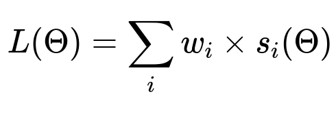
Here, L(Theta) is the total loss. Each s_i(Theta) measures a specific aspect like error against holdout data or discrepancy from experimental effect estimates. The w_i are weights that balance these terms.
Combining Sub-models Wrap all sub-models in a “ModelCollection,” which acts like a single composite model. The ModelCollection has:
A combined forward pass that routes each model’s output to the relevant subsequent inputs.
A combined training routine that orchestrates parameters across modules.
Backtesting and Causal Validity Checks Evaluate predictions by:
Backtesting on historical data.
Checking if predicted treatment effects align with known experimental results.
Using unit-agnostic error metrics (like MASE) to compare performance across metrics.
Decision Optimization Feed the validated model into an optimization routine that searches for the best input decisions to maximize or minimize an objective. For example, you might maximize total rides subject to cost constraints. In practice, you solve:
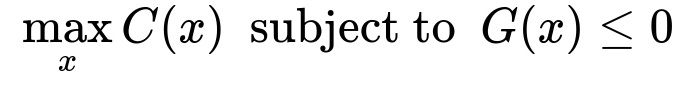
C(x) might be profit or number of rides. G(x) might encode constraints on budget, wait times, or prime-time levels.
If the model is differentiable, you can use gradient-based methods to handle high-dimensional inputs. This approach automates discovering the optimal settings (for instance, driver incentive spending by region and time).
Retrospective Evaluation Compare actual decisions to ex-post decisions that assume perfect foresight. If your model-based decision approach yields significantly worse outcomes than those ex-post optimal decisions, you measure that gap as regret:
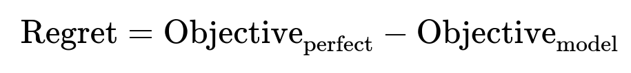
A high regret signals the system’s forecasts or assumptions need refinement.
Follow-up Questions and Exhaustive Answers
How do you ensure your sub-models remain causal in a real-world environment with confounding variables?
A data scientist must confirm each sub-model captures cause-effect relationships rather than pure correlations. One reliable way is randomized experiments. If an experiment shows X% change in input leads to Y% change in output, incorporate that result as a strong constraint on the model’s mapping. If experiments are not available, use domain knowledge and observational data combined with causal identification methods (instrumental variables, difference-in-differences, or structural assumptions). You confirm these sub-models by checking whether they can match known treatment effects when backtested on any prior policy shifts or A/B experiments.
How do you integrate domain-specific constraints (like budget limits) directly into the decision optimization?
Combine constraints in the objective function as soft penalties or use constrained optimization. When using gradient-based methods, one popular approach is projected gradient descent, which projects solutions back into the feasible set after each gradient step. Another approach is to add large penalty terms in the objective for constraint violations. Both approaches keep the problem differentiable and solvable with auto-differentiation. You also verify that each region’s budget, or each product line’s limit, is never exceeded by checking final solutions.
How do you handle the computational cost of training many sub-models and running optimization for high-dimensional decisions?
Partition the problem. Train each sub-model separately first with its own local data and metrics. Then assemble them into a model collection. If the DAG is large, schedule updates in segments or use distributed optimization. Caching is also essential. For example, precompute certain partial results or store repeated index operations. When optimizing decisions, gradient-based methods are efficient in high-dimensional continuous spaces, especially when sub-models share the same index structures.
How do you diagnose which sub-model is causing poor forecasts or flawed decisions?
Use the system’s modular design. Temporarily isolate each sub-model and compare predicted vs. actual outcomes for metrics it directly influences. Inspect the model’s partial derivatives to see how strongly an input influences a downstream metric. If that partial derivative is large, it might be a source of big forecast error. Also compare each sub-model’s predictions against known experiments or holdout sets. Once identified, fix or refine that sub-model with extra features, updated assumptions, or new experimental data.
How do you practically convince stakeholders that the final recommendations are trustworthy?
Explain each sub-model’s alignment with experiments. Demonstrate retrospective analyses showing low regret. Show how the system’s predictions line up with real business outcomes. Provide sensitivity analyses: for example, if the model is off by a certain percentage in driver behavior, how does that affect final decisions? Such analyses build confidence that the recommended decisions remain robust within realistic uncertainty ranges.
How would you extend this system if new data or a new product feature is introduced?
Modularity ensures that, if a new feature changes driver incentives, you add or replace a sub-model capturing that effect. Update the DAG so the new sub-model’s outputs link to downstream consumers. Re-run training procedures, verifying that each sub-model’s forward pass is still correct. If needed, gather new experimental data. Then re-run the end-to-end optimization. This incremental approach leverages the existing structure while integrating the new component with minimal disruption to other modules.
How do you handle unseen or rare events (for example, drastic changes in demand patterns due to unforeseen externalities)?
Build robust models that gracefully degrade. Techniques include hierarchical structures that rely on partial pooling across related categories or time periods. During optimization, apply constraint buffers to ensure decisions don’t overly rely on uncertain forecasts. If possible, keep a fallback or override mechanism that triggers a simpler rules-based approach if predictions become too uncertain. Meanwhile, gather new data whenever these rare events happen and incorporate them to improve future predictions.
How do you ensure the optimization is not over-fitting to short-term data patterns?
Use backtesting across multiple time windows and, if possible, block-based cross-validation. Ensure the loss function includes regularization terms that penalize unrealistic parameter values. Evaluate decisions with different historical slices to see if recommended actions vary wildly. If so, impose smoother constraints (for instance, limiting daily changes in incentives). Also run consistent holdout validations and watch if the model’s performance drifts significantly over time.
How do you debug gradient-based optimization if the solution fails to converge or gives erratic results?
Check if the loss function is too flat or too steep in certain regions. If the gradient is exploding, reduce the learning rate. If the gradient is vanishing, re-scale inputs or outputs. Ensure the indexes match properly so broadcasting occurs in expected dimensions. Inspect partial derivatives of each sub-model to identify anomalies. Add gradient clipping if needed. Sometimes switching to a different optimizer (Adam vs. SGD) or changing initialization can help. Also verify constraints are not so tight that the feasible region is nearly empty.
How do you measure the financial or operational impact of your final recommendations after deployment?
After making recommended decisions, measure actual outcomes and compare them to the model’s predicted outcomes. Compute regret by contrasting the model-based decision with an ideal ex-post decision that uses observed data. If the difference in objective is small, your system performed well. If it’s large, investigate which sub-model or assumption caused the largest error. Log all important metrics (driver hours, prime-time, profit) for retrospective reviews. Present these results to stakeholders to maintain confidence in the system and guide future improvements.