
ML Case-study Interview Question: Optimizing Recommendations within Time Budgets using Reinforcement Learning.


Browse all the ML Case-Studies here.
Case-Study question
A streaming platform wants to show a ranked list of recommendations to each user. Users have a limited time to evaluate each title, and they may abandon the search if their time is consumed before they find something appealing. The platform needs a system that combines relevance and time-cost of items so that users are more likely to pick a recommendation before running out of time. How would you approach this problem from a Machine Learning perspective? Suggest a data-driven solution to learn a policy that maximizes the probability of user engagement under finite time constraints. Propose specific modeling techniques and describe how you would handle both on-policy and off-policy scenarios.
Detailed solution
A budget-constrained recommendation system targets maximizing user engagement while keeping the total evaluation time of recommended items within the user's time budget. This is similar to a 0/1 Knapsack setup, where each item has a relevance (utility) and a time cost, and we try to pick items whose combined cost does not exceed the user's budget.
Many solutions use bandit approaches for slate recommendations, but they often do not explicitly consider the user’s available time. Reinforcement Learning (RL) is effective when we must balance multiple items with differing relevance and cost. The system can maintain a Q-function that estimates future rewards for each action (item selection) given the remaining time budget.
Formulating it as 0/1 Knapsack

Here:
S is the chosen subset of items in the slate.
beta_i is the relevance of item i.
c_i is the cost (time) of item i.
u is the user’s time budget.
The solution set must also consider ordering (higher relevance items earlier).
Markov Decision Process approach
The state can contain the remaining time budget and any necessary context about user preferences. The action is choosing the next item to recommend. The reward can be 1 if the user consumes an item or 0 otherwise. A discount factor gamma > 0 can help the system prioritize longer-term returns by packing more feasible items in the slate.
For each state, the Q-function q(s, a) estimates expected discounted reward. A temporal difference update can be used:
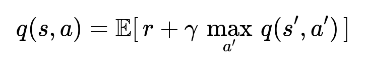
This is the core RL equation for Q-Learning. Training proceeds by sampling user sessions (real or simulated) and updating q(s, a) accordingly.
On-policy vs Off-policy
On-policy methods like SARSA collect experiences while following the current policy. Off-policy methods like Q-Learning learn from data generated by a different policy. Off-policy learning is essential in large-scale recommenders because production data often comes from older policies. The main difference is that off-policy methods use the optimal action in the next step for the value update, whereas on-policy methods use the actual action taken in the next step.
Practical implementation details
A model can approximate q(s, a) with a neural network. Inputs would include user features, item features, and the remaining time budget. The output would be the expected return for each possible action. The top Q-value items that fit the cost constraint can be shown first. Training requires a dataset of (state, action, reward, next state) tuples. The system can retrain periodically, or refine the Q-function in an online fashion if real-time feedback is available.
Example code snippet
import torch
import torch.nn as nn
import torch.optim as optim

class QNetwork(nn.Module):
    def __init__(self, state_dim, action_dim):
        super(QNetwork, self).__init__()
        self.fc1 = nn.Linear(state_dim, 128)
        self.fc2 = nn.Linear(128, 64)
        self.fc3 = nn.Linear(64, action_dim)

    def forward(self, x):
        x = torch.relu(self.fc1(x))
        x = torch.relu(self.fc2(x))
        x = self.fc3(x)
        return x

# Suppose we have a minibatch of transitions
def q_learning_update(q_network, optimizer, transitions, gamma):
    states, actions, rewards, next_states, done_flags = transitions

    # Compute current Q-values
    q_values = q_network(states)
    q_current = q_values.gather(1, actions.unsqueeze(1)).squeeze(1)

    # Compute target Q-values
    with torch.no_grad():
        q_next = q_network(next_states).max(1)[0]
        q_target = rewards + gamma * q_next * (1 - done_flags)

    # Loss
    loss = nn.MSELoss()(q_current, q_target)

    optimizer.zero_grad()
    loss.backward()
    optimizer.step()
The code uses a simple Q-Learning loss. The q_current is the Q-value for the taken action, and the q_target is the observed reward plus the discounted maximum next Q-value. The time budget factor would be part of the state.
Follow-up question 1
How do you handle unknown or unobservable time budgets during training and inference?
Explanation
Some users’ exact time budget is not directly measured. One approach is to infer a hidden budget from historical engagement signals, such as how long a user scrolls before abandoning. A simpler method is to assume a distribution over budgets and sample from that in a simulation. Another approach is building a latent variable model, learning an embedding for budget from usage patterns. During inference, the system can maintain a distribution over possible budgets and select items accordingly.
Follow-up question 2
Why might RL outperform a simpler contextual bandit approach when time is limited?
Explanation
A contextual bandit model greedily picks items based on immediate reward estimates. It does not factor in how each chosen item’s cost reduces the user’s remaining time. An RL approach explicitly models how choosing a higher-cost item can reduce overall returns if it crowds out other feasible items. RL agents learn to pick a balance of items that maintain a higher chance of engagement.
Follow-up question 3
Why does Q-Learning yield different effective slate sizes compared to SARSA?
Explanation
SARSA updates the Q-function based on the next action actually taken by the current policy, so it can promote more cautious exploration. Q-Learning updates based on the greedy best next action, which can lead to different learned policies. Large effective slates from Q-Learning may indicate that the agent exploits certain patterns to maximize coverage of feasible items, whereas SARSA tries to adapt to the actual policy’s next step, resulting in a different set of trade-offs.
Follow-up question 4
How do you evaluate and compare RL policies in a real production environment without risking a poor user experience?
Explanation
One method is off-policy evaluation using logged data. In such a pipeline, you use historical (state, action, reward) logs from the old policy and estimate the new policy's performance by applying importance sampling or other off-policy estimators. Another approach is A/B testing, gradually rolling out the new policy to a fraction of users. If metrics like engagement or completion rate improve, you increase its share. Safe thresholding can ensure no severe drops in performance.
Follow-up question 5
How would you extend this method for larger item catalogs and more complex user states?
Explanation
Scaling to larger item sets requires approximate methods for item selection. You can rank items by Q-value and then filter them by cost constraints. You can also use a multi-level approach, first selecting a subset of items via approximate search or retrieval, then ranking that subset with the RL model. More complex user states can include additional features like time-of-day, device type, and past watch history. Neural architectures can handle these richer inputs, but careful feature engineering and distribution shift monitoring are critical.
Follow-up question 6
What hyperparameters or design choices might be crucial in practice?
Explanation
Discount factor gamma controls the trade-off between immediate reward and future reward. Learning rate affects the stability of updates. Exploration strategy (epsilon-greedy or more sophisticated methods) can change the variety of items served. Representation learning for item features and user states can heavily impact system performance. In real systems, you must also handle data staleness, delayed rewards, and item changes (new content added, old content removed).
Follow-up question 7
How would you manage cold-start items or users with no known time budget or relevance signal?
Explanation
Exploration is essential. The model can reserve a few slots for new items or new users, either by random sampling or contextual uncertainty-based methods. You can bootstrap the cost and relevance estimates from content metadata or user demographics. As more data arrives, the RL agent refines these estimates. Bayesian approaches or Thompson sampling can help handle uncertain budget distributions for new users.
Follow-up question 8
Could other resources replace time as the central budget in the algorithm?
Explanation
Yes. Any finite resource (money, screen space, network constraints, etc.) can fit the same approach. If the user has limited attention or partial connectivity, an RL-based method can weigh item cost (like data size or subscription cost) against relevance. The main idea remains to pick items that maximize long-term reward without depleting a crucial resource.
Follow-up question 9
Why might a sequential slate construction process (one slot at a time) be preferred over a static approach?
Explanation
It offers flexibility to incorporate intermediate feedback and context. If the user partially consumes some content or reveals more preferences, the algorithm can adapt the later slots. It can also help in simulation-based training, where the agent updates the next choice based on the user’s simulated response and remaining budget. Some methods compute the entire slate simultaneously, but a sequential approach often integrates well with standard RL paradigms.
Follow-up question 10
What key implementation pitfalls do you foresee when deploying such RL-based recommenders?
Explanation
Overestimating Q-values is common if the algorithm updates are unstable. Distribution shift arises if the policy changes rapidly and historical data becomes obsolete. The neural net might need significant regularization. Offline logs may not reflect real user budgets accurately. Balancing exploration vs exploitation is tricky at scale, and partial observability of user states or budgets can introduce bias if not accounted for properly. Frequent validation with holdout sets and careful monitoring in production helps mitigate these issues.