ML Case-study Interview Question: Stage-Wise Neural Networks for Accurate Real-Time Food Delivery ETA Prediction.

Browse all the ML Case-Studies here.

Case-Study question

A large-scale food ordering and delivery platform wants to improve the accuracy of its Estimated Time of Arrival (ETA) predictions. They break down the journey into four stages: Ordered to Assignment (O2A), First Mile (FM), Wait Time (WT), and Last Mile (LM). The platform must incorporate real-time signals like restaurant workload, driver location updates, and potential traffic disruptions. The business goal is to reduce customer anxiety from sudden large jumps in ETAs and keep the Mean Absolute Error within a low threshold. Propose a full system solution that addresses data collection, model design, training approach, and evaluation metrics. Suggest ways to handle real-time updates and model improvements over time. Provide a comprehensive approach and reasoning.

Detailed Solution

Stage-Wise Architecture

Each order’s journey is divided into four segments. O2A covers the time until a driver is assigned. FM covers pickup travel time. WT covers waiting time at the restaurant. LM covers travel time from pickup to drop. Different features are relevant in each segment. For example, LM heavily depends on traffic patterns, so real-time driver pings and speed calculations become critical.

Real-Time Distance and Speed Features

Accurately measuring distance is central to predicting travel time. The system calculates haversine distance between pings to estimate how far the driver has already traveled and how fast they are moving. It also calculates the distance from the driver’s current position to the customer location. Below is the core formula for the haversine distance:

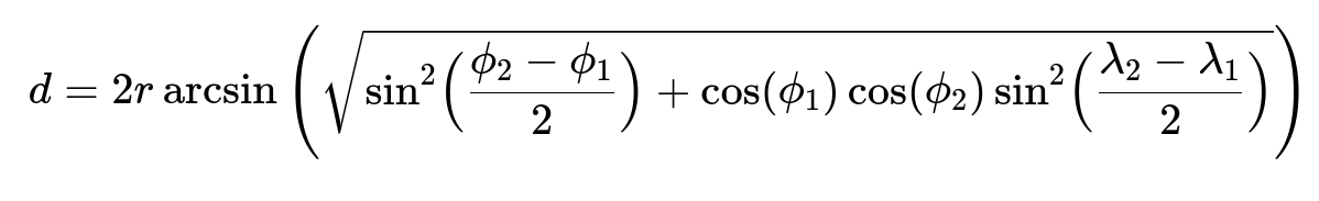
r is the Earth’s radius. phi_1 and phi_2 are the latitudes in radians, and lambda_1 and lambda_2 are the longitudes in radians. The system sums these distances between consecutive pings over short time windows. Dividing total distance traveled by the time in that window yields an estimate of real-time speed, which helps adjust ETAs dynamically.

Evaluation Metrics

The main metric is Mean Absolute Error (MAE). The system monitors how closely predictions match actual delivery times:

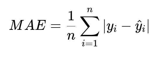
n is the total number of orders. y_i is the actual delivery time, and hat{y}_i is the predicted delivery time. The platform tracks “inaccurate bumps” in real time as well. If a sudden jump in ETA is large enough and wrong, it raises red flags and erodes user trust.

Modeling Approach

A Gradient Boosting Tree (GBT) model with absolute loss was initially used. It gave significant improvements over legacy estimates. However, GBT predictions can be less flexible when the environment changes quickly. To address those concerns, the system shifted to Neural Networks.

Four neural networks each manage O2A, FM, WT, and LM. For instance, the LM model has hidden layers that process real-time pings, speeds, and distances. Neural networks are trained for multiple epochs with an ADAM optimizer. Each network’s architecture includes several fully connected layers with Leaky ReLU activation.

Below is a short Python snippet illustrating how a training script might look:

import tensorflow as tf
from tensorflow.keras import layers, optimizers

# Example architecture for LM stage
model = tf.keras.Sequential([
    layers.Dense(8, activation='linear', input_shape=(input_dim,)),
    layers.LeakyReLU(alpha=0.01),
    layers.Dense(8),
    layers.LeakyReLU(alpha=0.01),
    layers.Dense(8),
    layers.LeakyReLU(alpha=0.01),
    layers.Dense(1)  # Final output: predicted ETA in minutes
])

model.compile(optimizer=optimizers.Adam(learning_rate=0.001),
              loss='mae',
              metrics=['mae'])

model.fit(train_data, train_labels, epochs=50, validation_split=0.1)

The shift to neural networks raised accuracy by about 15 percent and lowered inaccurate bumps by 12 percent compared to GBT, boosting customer trust.

Handling Real-Time Updates

The system reassesses predictions whenever new data arrives (e.g., new driver pings). The neural network reevaluates conditions and updates ETA. When certain triggers occur (like unexpected high restaurant stress or road closures), the model can respond faster to keep ETAs realistic. In some cases, big jumps are necessary but the system must confirm correctness with features indicating any new disruptions.

Future Enhancements

Sequence models, like RNN or LSTM, can help when distance and speed data must be learned over a series of time steps. Graph Neural Networks can strengthen the representation of complex street networks, especially for the LM stage. Additional features, such as points of interest or driver rejections, help handle outlier cases.

Possible Follow-Up Questions

1) How would you handle sudden driver behavior changes, such as unplanned stops?

Neural networks need robust real-time features. If a driver is stationary beyond a small threshold, the system incorporates a higher wait penalty. Updating the input vectors to the model with frequent pings ensures the output captures that stationary delay quickly. A fallback rule-based component could catch extreme outliers: for instance, if the driver has not moved for a prolonged period, an additional offset is added, and the model is retrained with these examples so it learns from real cases.

2) Why not rely on a single global model for all segments instead of separate ones?

Each segment demands unique features. O2A depends on how quickly the system assigns a driver. FM involves route data from restaurant location to the pickup point, while WT focuses on time spent waiting at the restaurant. LM heavily relies on traffic-based speed features. A single global model risks mixing these signals and diluting specialized feature sets. Separate models allow deeper optimization per stage.

3) Why is MAE chosen over other metrics like RMSE?

MAE correlates directly to the magnitude of error in minutes. Customers experience lateness or earliness in linear terms. MAE penalizes each minute of error equally. RMSE penalizes larger errors more. In a real-world setting, a few outliers should not overshadow overall performance. MAE is simpler to interpret. Additionally, the platform monitors inaccurate jumps as another metric to track abrupt changes.

4) How would you handle training at scale with constant data inflow?

A pipeline that continuously ingests new data is essential. Periodically retrain models using streaming updates. Maintain rolling windows of data to capture recent trends. For fast iteration, a well-structured MLOps pipeline can automate data validation, model retraining, and deployment. Online learning approaches might also be tested for near-instant adaptation.

5) What if neural networks overfit or degrade in production?

Regularly measure holdout performance. Keep an eye on metrics like MAE. If overfitting occurs, incorporate regularization like dropout or weight decay, or reduce hidden layer sizes. For production drift detection, set up alerts that fire if real-time MAE goes beyond the expected range. This triggers investigations or fallback to previous stable models until fixes are deployed.

6) How would you integrate sequence models like LSTM for further improvements?

Treat driver pings as a sequence. Feed each ping’s coordinates, speed, and timestamp into an LSTM or GRU. The recurrent cell tracks patterns over time. This can reveal velocity trends or repeated stops. The final hidden state can output the predicted remaining time. Sequence models handle time-series data more naturally. They also adapt better to variable route durations.

7) Why consider Graph Neural Networks for the LM stage?

Road networks and traffic patterns form a graph structure: intersections are nodes, streets are edges. GNNs learn relationships between connected locations. They can capture how congestion in one region impacts adjacent roads. This approach handles localized traffic surges better. If the graph is large, sampling or hierarchical GNN methods might be used to keep training efficient.

---