
ML Case-study Interview Question: Predicting Reliable Food Delivery ETAs Using XGBoost Regression

Browse all the ML Case-Studies here.
Case-Study question
A popular online food delivery platform faces high order volumes daily. They observe that overall waiting time strongly affects user satisfaction and conversion rates. They decide to build a system (called Tensoba) to predict the Estimated Time of Arrival (ETA) from the moment a user places an order until the food is delivered. The system outputs its ETA in two stages: ETA Discovery (shown before checkout) and ETA Checkout (shown at checkout). The aim is to keep the prediction close to the actual delivery time (Actual Time of Arrival, ATA).
They collect large-scale historical data, including merchant-level information (average cooking durations, location) and order-level information (traffic, distance, total order value). They want the predictions to be accurate, to avoid overestimations (which reduce conversions) and underestimations (which reduce user trust).
Question: As a Senior Data Scientist, outline your solution strategy to design and deploy a system that provides reliable ETAs for each order. How will you ensure the accuracy of these predictions? How will you handle large-scale data with many merchants and varied order details?
Proposed In-Depth Solution
Framing the Problem This task is a regression problem predicting a continuous numeric target (time in minutes or seconds). Directly modeling the entire arrival time as a single output is feasible, but splitting it into separate components often yields better accuracy. The components can be:
Time from order creation to driver arrival at the restaurant (T1).
Time from driver arrival at the restaurant to driver pickup (T2).
Time from driver pickup to delivery completion (T3).
Adding up T1, T2, and T3 yields the final ETA. Another approach is to train a single model that predicts the total ATA directly.
Model Inputs
Merchant-level features can include historical averages, standard deviations, or percentiles of preparation times. Order-level features can include the number of items, total order value, and real-time route distance.
Offline Metrics
They measure error with three metrics:
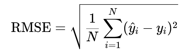
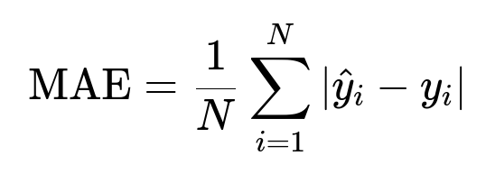
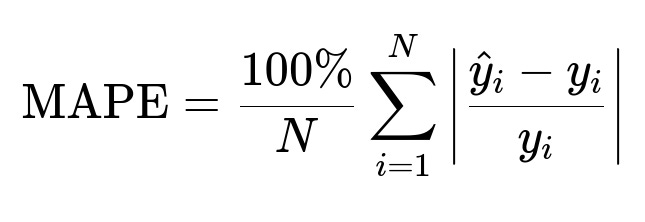
Here, y_i is the true arrival time, and hat{y}_i is the predicted arrival time.
They choose RMSE if large errors must be penalized more. They choose MAE if all errors must be penalized equally. They choose MAPE to measure the percentage difference between prediction and actual time.
Online Metrics
They evaluate:
Compliance: The fraction of orders where the actual arrival does not exceed the predicted time by too much. Over-promising reduces user trust.
Conversion: The fraction of user sessions that result in a completed order. Overly high ETA predictions discourage ordering.
Baseline Approach
They first try a simple historical average for each merchant. This yields about 6 to 7 minutes average error and ~32% MAPE. They aim to beat this baseline.
Modeling Approach
They build separate models for (T1, T2, T3) or a single model for the entire ATA. They train these using XGBoost on a few weeks of data. They gather features like:
Merchant-level average T1 or T2 during specific hours over recent days.
Distance group for T3 (longer distances yield longer T3).
Order value or item count.
The final predicted ETA for a single order can be:
T1 + T2 + T3 from three specialized models, or
Direct prediction from one model for total ATA.
They observe that separate models often give better accuracy because T1, T2, T3 depend on different factors.
Implementation
They run batch predictions for T1 and T2 every hour. These components do not require highly individualized user features. They store them in a key-value storage for quick retrieval by the application.
They deploy real-time predictions for T3 at checkout. This uses an API that fetches current order details (distance, items) and calls the model to return an updated T3. They sum up T1 and T2 from batch outputs with the real-time T3.
They use feature stores to retrieve merchant and location data. They rely on a real-time inference service that loads the XGBoost model, processes features, and returns predictions within milliseconds.
Model Performance
They see that combining T1 + T2 + T3 prediction models reduces the MAPE from around 31% to 23%. This indicates users see more reliable ETAs.
They notice top features for T1 and T2 revolve around past performance of the same merchant at that hour. For T3, distance strongly influences travel time, along with location-based historical data (like average traffic conditions in certain areas).
Future Improvements
They plan continuous retraining with the latest data. They also plan to incorporate live signals about restaurant crowds, or real-time driver acceptance behaviors. They may extend to advanced algorithms or update features more frequently to handle dynamic scenarios.
They gather frequent feedback from A/B tests to check user satisfaction and track whether compliance and conversion targets are met.
What if…
1) The real-time feature store has occasional lags. How would you ensure data freshness?
Answer: The system must have consistent updates and robust data pipelines. A short caching window is acceptable, but data older than a few minutes might lead to stale features. One way is to keep a time-to-live on cached features. If data is too old, the fallback might be default values. Another approach is to maintain real-time ingestion from streaming systems and verify the pipeline with checksums or data-latency alerts. The team might separate critical features that must be fresh from less time-sensitive features updated hourly.
2) Many merchants have sparse data because of fewer orders. How do you handle these cases?
Answer: One approach is to cluster merchants with similar profiles and pool their historical data. Another approach is to backfill missing features with overall averages or regressions. Regularization helps prevent overfitting to minimal data. The model can use transfer learning from merchants with extensive data to those with limited data. They can also build hierarchical features (city-level or region-level) to fill gaps.
3) How would you handle zero or near-zero actual arrival times when calculating MAPE?
Answer: We must avoid division by zero. One solution is to filter out or adjust zero-time records (they might be data errors). Another is to use a different error metric for those edge cases. Some teams add a small offset to the denominator. If zero times are invalid data points, they are removed during training. If they are legitimate edge cases (such as pre-packaged items), the pipeline might rely on MAE or RMSE to avoid that pitfall.
4) How do you deal with outliers that skew model performance?
Answer: Large outliers often happen due to events like driver cancellations or extreme traffic. They can be capped or transformed using logs. They can be weighted less during training. The team can train on typical ranges but keep a separate mechanism to handle extreme events. Monitoring outliers helps the team refine data filters and possibly route those orders differently.
5) Why choose XGBoost over deep neural networks?
Answer: XGBoost is faster to train, easier to interpret, and handles tabular data well. Sparse merchant data might not benefit from deeper models. XGBoost also handles missing values gracefully and offers fine control over regularization. If the data were very high-dimensional or mostly unstructured, a neural approach might be helpful. In practice, gradient boosting trees often outperform deep networks for structured tabular problems.
6) How would you ensure that the new ETA system does not hurt conversion?
Answer: The team runs A/B experiments. A control group uses the old ETA, and the treatment group uses the new ETA. They measure the difference in conversion and compliance. If conversion dips, they check whether the new model is overestimating or underestimating. They adjust the model or calibrate the outputs to find an acceptable trade-off. They might incorporate a slight buffer to reduce the risk of underestimation.
7) How do you scale the batch predictions for thousands of merchants hourly?
Answer: They schedule distributed jobs that load the trained model, run inference for all merchants in parallel, and store results in a high-throughput data store. Cloud-based orchestration tools manage dependency and resource allocation. They might partition data by region or merchant segments to process more efficiently. They ensure they can handle concurrency with robust parallelization and cluster autoscaling.
8) How would you validate the reliability of the model in production?
Answer: They would maintain real-time logging of predicted vs. actual times and compute error metrics continuously. They set automated alerts if metrics degrade. They would systematically compare short-term average performance with offline validations and run near-real-time dashboards. They might store the model’s predictions, ATA events, and user feedback to analyze mispredictions and refine features.
9) How do you handle the cold-start problem for new merchants?
Answer: They might default to a global or regional average for T1, T2, T3 until enough data accumulates. They can also leverage merchant similarity features to approximate cooking times. As soon as a new merchant starts getting orders, the system updates partial aggregates and transitions gradually from the default to the merchant-specific model outputs.
10) How would you incorporate driver acceptance probability?
Answer: They would train a sub-model to estimate the probability of immediate driver acceptance. That probability can shift T1. If acceptance is less likely, T1 might spike. They could feed acceptance probability or expected wait times for driver allocation into the main model. They could store driver acceptance trends per region, time of day, or merchant segment. This factor helps refine the overall ETA, especially when driver availability is uneven.