
ML Case-study Interview Question: Optimizing Real-Time Delivery Dispatch Using Machine Learning and Mathematical Optimization


Browse all the ML Case-Studies here.
Case-Study question
A large on-demand delivery platform operates a three-sided marketplace consisting of merchants preparing food or goods, customers placing orders, and drivers fulfilling delivery requests. Each incoming order must be assigned to the most suitable driver to ensure rapid deliveries and minimize driver downtime. The platform seeks a system that can:
Predict real-world conditions for each order, including preparation time at the merchant, travel time from the driver to the merchant and then to the customer, and the likelihood each driver will accept the order.
Use those predictions within a mathematical optimization framework to decide which driver should be assigned each order, and also to decide whether multiple orders might be batched (handled by one driver simultaneously) for efficiency gains.
Continuously improve through simulation and experimentation, because marketplace conditions vary across geographies, demand fluctuations, weather changes, and many other external factors.
Design and explain a data science solution that uses machine learning models and an optimization approach to address the above objectives in real time. The system should also account for uncertainty in the model estimates, avoid overfitting, and be robust to changing patterns in driver or user behavior.
Detailed Solution Explanation
Overview of the Dispatch Engine
The system first collects incoming orders, drivers’ current states (busy, available, or finishing another delivery), and any known external signals such as weather. It then constructs potential driver-order assignments, scores each possibility with a set of machine learning (ML) models, and finally chooses the assignments through a mixed-integer optimization model. The engine repeats this process on a rolling basis, updating the marketplace state as new orders arrive or drivers complete tasks.
Machine Learning Layer
The machine learning layer focuses on three core predictions: the time until each order is ready for pickup, the travel time for a driver to reach the merchant and then to deliver to the customer, and the acceptance likelihood for each driver-order pairing. A preparation time model estimates when the merchant will have the order ready. A travel time model estimates how long it takes a specific driver to get from their current location to the merchant and then to the customer. A driver acceptance model predicts if the driver will accept or reject the proposed order, which helps the system avoid repeatedly offering the same order to drivers who are unlikely to accept it.
Historical data (orders, driver positions, merchant speeds) serves as input to train these models. Each model might use gradient boosting or neural networks, though simpler naive averages for specific merchants or segments can still capture certain patterns (such as average wait time for parking). This layer outputs the best estimates for each key metric.
Optimization Layer
An integer or mixed-integer programming (MIP) model incorporates these ML predictions to produce final assignments. The optimization engine scores each potential assignment based on metrics such as expected total delivery time, predicted driver acceptance, and lateness risk. Batching possibilities are also included as separate candidate assignments. Batching can reduce overall travel if multiple orders have similar pickup or dropoff zones.
A common formulation is to minimize total cost or lateness while respecting constraints like driver availability, order deadlines, and assignment exclusivity. A simple version of the objective might look like this:
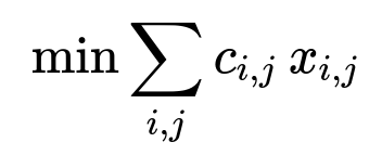
Where i enumerates orders, j enumerates drivers, c_{i,j} is a cost metric for assigning order i to driver j (travel time, lateness risk, or a combination), and x_{i,j} is a binary variable that equals 1 if order i is assigned to driver j and 0 otherwise. Constraints ensure each order is assigned to exactly one driver (or a small set of potential batched routes) and that drivers have feasible routes in terms of time and location. Batching logic extends the formulation to allow a driver to handle multiple orders, adding route sequencing constraints and additional cost terms for complex multi-stop routes.
Accounting for Model Interactions and Variability
The ML models’ outputs become inputs to the optimization. Overly biased predictions degrade solution quality; poor estimates cascade into suboptimal assignments. The system mitigates this risk by regularly retraining ML models using rolling windows of data, carefully tracking drift in real-time. Overfitting is addressed by employing parameter tuning strategies like Bayesian optimization, which tunes optimization model coefficients (for example, how heavily to weight time vs. cost vs. acceptance rates) without locking the system into a local optimum. The solution also penalizes complexity if too many stops or uncertain parameters might lead to wide deviations in actual delivery times.
Simulation and Experimentation
Simulation provides a low-risk sandbox for testing changes to the ML or optimization layers. Synthetic events replay historical data while altering specific conditions (demand surges, driver shortages, weather disruptions) to see how the proposed assignment logic behaves. Experimentation in production uses specialized designs (like switchback tests) to handle network effects, randomly assigning different configurations to certain regions or time windows. Analyzing results with variance reduction techniques and robust standard error estimates gives reliable insights about the net impact of each model change.
Example Code Snippet for Simple Parking Time Estimation
import pandas as pd
import numpy as np

# Suppose historical_parking_times is a DataFrame with columns: store_id, parking_time
def estimate_parking_time(store_id, historical_parking_times):
    subset = historical_parking_times[historical_parking_times.store_id == store_id]
    if len(subset) > 0:
        return np.mean(subset.parking_time)
    else:
        return np.mean(historical_parking_times.parking_time)  # fallback average
This snippet shows a basic way to generate naive estimates that feed into the broader travel time model.
Continuous Improvement
The combination of ML modeling, real-time optimization, simulation, and experimentation allows the platform to adapt daily. Retraining on fresh data preserves model quality. Refined optimization parameters (for instance, better weighting of acceptance risk) improve resource usage. Simulation explores hypothetical supply-demand imbalances before they occur. Experimentation ensures that any new approach is tested on real data in controlled conditions, so the system’s performance remains strong and stable.
How to Answer Follow-up Questions
Below are possible follow-up questions an interviewer might pose, each followed by a detailed discussion of how to approach them.
1) How would you handle driver acceptance rates and prevent repetitive offers to drivers?
Driver acceptance likelihood is predicted in the ML layer. This probability influences the optimization layer by raising the expected cost of assignments that a driver is likely to reject. A method is to include a penalty factor for repeated offers of the same order. The system attempts the highest-probability match first; if that driver rejects, the cost for offering to them again becomes even higher. This approach is calibrated using historical acceptance data and updated regularly. The system measures how many offers are typically needed until an order is finally accepted, and it identifies any driver or time-window segment that systematically declines certain orders.
2) How do you avoid overfitting the optimization parameters?
Parameter overfitting often arises from tuning the system to historical data that may not match future conditions. Bayesian optimization is a good choice to balance exploration of parameter space with performance. By sampling parameter combinations in simulations or small-scale experiments and updating a posterior belief of how each combination performs, the system adapts to new data distributions. Regularization in the ML models also helps, but a separate approach is required for the MIP parameters that combine those predictions into an assignment decision. The solution is to keep a wide range of test scenarios in simulation, exposing the tuning process to unusual data segments so the final parameter set is robust.
3) What steps do you take to manage cascading variability?
Every ML output has uncertainty, especially for complex or longer routes. The optimization model incorporates a variance penalty for each route. If a batch route has uncertain preparation times at multiple restaurants, that might expand the route’s total time window unpredictably. The system increases the cost term for uncertain routes to reduce unexpected delays. This penalty can be dynamically scaled according to the standard deviation of predicted times, so the system remains flexible but avoids risking extreme lateness on highly uncertain assignments.
4) How do you handle real-time changes in the marketplace, such as new orders arriving or drivers going offline?
Dynamic dispatch is essential. The optimization engine periodically (or continuously) re-solves the assignment with the latest data on driver states, order statuses, and updated ML predictions. At each iteration, the system checks if a partially assigned route has become suboptimal due to new orders or changed driver availability. In some situations, it may wait before dispatching if the best driver is finishing another order soon. This tradeoff is decided by penalizing excessive wait times and lateness but rewarding better matches. The system also re-queries the ML layer for fresh preparation time predictions if a merchant runs behind schedule.
5) How do you validate proposed improvements before rolling them out?
Extensive simulation measures impact in controlled, but realistic, scenarios. Simulation helps quickly evaluate whether the optimization or ML tweak worsens the situation under certain conditions. Promising changes move to production experiments using region-based or time-based switchback testing to isolate the treatment group and measure top-line metrics such as average delivery time or driver utilization. The experiment’s data is analyzed for network effects, standard errors, and any segment-specific shifts. A final go/no-go decision is made after verifying the changes consistently boost metrics without introducing unacceptable side effects.