
ML Case-study Interview Question: Measuring Long-Term Notification Impact on E-commerce Retention via Causal Inference.

Browse all the ML Case-Studies here.
Case-Study question
A large e-commerce platform has many high-value users. They frequently purchase but can suddenly drop their purchase frequency. The Data Science team built a predictive model to flag potential churners and decided to intervene with a special discount notification in their mobile app to retain user engagement. Months later, the team discovered that measuring the real long-term impact of these notifications on purchase frequency and revenue is difficult because the effect is diluted over time. Design an end-to-end solution to measure the true incremental effect of these interventions on user retention. Propose how to structure A/B tests (RCT), tackle low acceptance of notifications, handle observational data, and perform robust causal inference. Include recommendations on measuring incremental value across time horizons, building meta-learners or regression-based estimators, and validating estimator robustness.
Detailed Proposed Solution
Randomization eliminates many biases, but a small fraction of users actually interacts with the notification, weakening statistical power in the long term. Splitting users into a test and control group ensures a fair baseline. When acceptance is very low, an observational approach is needed. Matching test users who actually take the offer with a comparable control group requires adjusting for confounding variables like past frequency or other behavioral signals.
Randomized Controlled Trials
Users are randomly assigned to test or control. Past covariates balance out across groups. The ideal metric is the Average Treatment Effect (ATE).
Here, Y(1) is the outcome (purchase frequency or revenue) if treated. Y(0) is the outcome if not treated. E[...] is the expected value over the distribution of users. This random assignment is powerful when acceptance rates are moderate to high, ensuring differences reflect actual treatment effects.
Handling Partial Compliance with Instrumental Variables
Some users in the test group never see or open the notification. Observing the sub-population that truly receives the treatment is necessary. The Complier Average Causal Effect (CACE) helps in these scenarios if certain conditions hold. In practice, the link between random assignment and actual treatment uptake can weaken over time, making results unreliable for long-term measurement.
Observational Study for Long-Term Analysis
Focusing on persuaded users requires conditioning on who actually took the treatment. Random group assignments no longer hold because users with higher purchasing behavior might interact more with notifications. Confounders must be identified and adjusted.
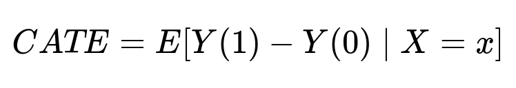
CATE is the Conditional Average Treatment Effect for users with features X. Estimating it requires methods such as inverse probability weighting, regression adjustment, or meta-learners (S-learner, T-learner, X-learner). Choosing the best estimator demands internal experimentation and rigorous checks.
Estimator Selection and Validation
An estimator must remove bias from differing user segments. Some estimators produce unreasonably large or small effects if the data is highly skewed. Meta-learners fit flexible models for Y(1) and Y(0) to generate stable estimates. Evaluations can include placebo tests, random common-cause injections, or dummy outcomes to confirm the estimator’s validity.
Example Code Snippet (Python)
import numpy as np
import pandas as pd
from sklearn.ensemble import GradientBoostingRegressor

# data has columns: ['user_id', 'treatment_flag', 'past_frequency', 'outcome']
# treatment_flag = 1 if user took the offer, 0 otherwise
# outcome is future purchase frequency

df = pd.read_csv('user_data.csv')

# Simple T-learner approach:
# Step 1: Split dataset by treatment_flag
treated = df[df['treatment_flag'] == 1]
control = df[df['treatment_flag'] == 0]

# Step 2: Fit separate models
features = ['past_frequency']  # plus any other covariates
model_treated = GradientBoostingRegressor()
model_treated.fit(treated[features], treated['outcome'])

model_control = GradientBoostingRegressor()
model_control.fit(control[features], control['outcome'])

# Step 3: Predict counterfactuals
df['y_hat_treated'] = model_treated.predict(df[features])
df['y_hat_control'] = model_control.predict(df[features])

# Step 4: Calculate individual-level effect
df['cate_estimate'] = df['y_hat_treated'] - df['y_hat_control']

# Summarize effect
average_effect = df['cate_estimate'].mean()
print("Estimated CATE:", average_effect)
Practical Considerations
No single estimator always wins. Real user behavior in a marketplace can be volatile. Combining domain knowledge with multiple modeling approaches is crucial. Adjusting for confounders like device type or purchase history is vital. After selecting a method that captures consistent effects in repeated experiments, validate its stability under stress tests.
Follow-up question 1
How can you ensure that historical purchasing behavior, device type, and other variables do not introduce bias into your observational results?
Answer
In observational analysis, stratifying or matching on confounding covariates ensures fair comparisons. If historical purchasing behavior correlates with both treatment uptake and future outcomes, ignoring it inflates the effect estimate. Constructing a propensity score to estimate the probability of treatment given past frequency, platform usage, and other variables reweights the control group so it resembles the treated group. Checking balance metrics (like standardized mean differences) before and after weighting confirms success. Running separate analyses for key subgroups (e.g., iOS vs Android) also reveals if there are unobserved interactions.
Follow-up question 2
What do you do if you find that two different causal estimators (e.g., T-learner vs IPW) give conflicting results for the same dataset?
Answer
Compare consistency of estimates across multiple experimental splits. Check if each method meets its assumptions (like positivity or no unobserved confounders). Review if there is a strong alignment between predicted propensity scores and the actual distribution. If T-learner has wide variance, refine hyperparameters or feature engineering. If IPW struggles with extreme weights, trim outliers or regularize propensity. Select the approach that shows stable estimates in repeated experiments. Verify with placebo treatments and synthetic tests. The method showing the most consistent alignment with domain expectations and placebo results typically prevails.
Follow-up question 3
How do you measure if the chosen approach remains valid over a longer horizon, given that user behavior can shift drastically over months?
Answer
Segment data by time windows and re-estimate effects. Compare early-window estimations with later-window estimations. If the same estimator loses consistency or produces implausible results, investigate shifts in user patterns or confounders. Retrain predictive models on fresh data reflecting seasonal and behavioral shifts. Track acceptance rates and re-check whether randomization or observational assumptions still hold. Validate with partial holdout groups. If results drift, adapt the model or redesign the experiment to capture emerging patterns.
Follow-up question 4
What steps would you take to communicate the final estimated incremental revenue to business stakeholders who want a single aggregate figure?
Answer
Aggregate the user-level or subgroup-level estimates to compute a total effect. Show the steps: from raw differences to adjusting for confounders. Highlight that the final figure is an expectation based on robust modeling. Provide best-case and worst-case intervals reflecting uncertainty. Demonstrate repeated experiments or placebo checks to build confidence. Offer actionable insights on which sub-populations benefit most. Maintain transparency on potential biases, stating that the model is recalibrated if user behavior changes.