
ML Case-study Interview Question: Two Tower Retrieval with LogQ Correction for Large-Scale Property Recommendation.


Browse all the ML Case-Studies here.
Case-Study question
A large travel platform gathers millions of property-search impressions, where each impression includes which properties were displayed, how many were clicked, and other context features. They need a high-performing candidate retrieval model to handle a huge inventory of properties. Using a Two Tower approach for retrieval, how would you design, train, and deploy this system, considering in-batch negative sampling, logQ correction, approximate nearest-neighbor search, and other hyperparameter decisions? Explain how you would process data at scale, train the model, handle negative sampling intricacies, apply the logQ correction, evaluate the system, and finally set up a production-ready retrieval pipeline.
Detailed solution
Building a two-stage recommendation pipeline is the aim, with a candidate retrieval step that narrows down to the most relevant items and a ranking step that sorts those items with more expensive algorithms. A Two Tower candidate generation model encodes user/context features in one tower and item features in another. A dot product between these embeddings measures relevance.
Data processing
Data includes user impressions with click labels. Filtering on clicked items produces a training set of positive examples. In a big-data environment, PySpark is suitable for distributed processing of user interactions. A critical preprocessing step involves counting how often each item appears. Dividing by total interactions produces a sampling probability for each item, used later for logQ corrections.
Saving data as TFRecord files is common for ingestion into TensorFlow, since it allows efficient streaming of large data into training. Each record holds all relevant features (user, item, label, sampling probability).
Model structure
A user tower maps user/context features to a D-dimensional vector. An item tower maps candidate features to the same D-dimensional space. Each tower is usually a stack of dense layers with nonlinear activations.
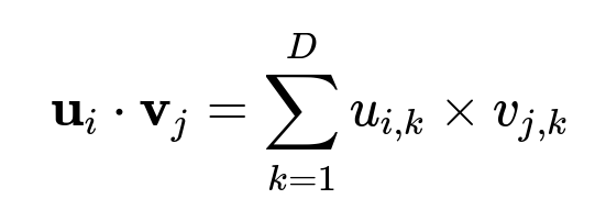
The vector u_i is the user embedding from the first tower. The vector v_j is the item embedding from the second tower. D is the embedding dimension. The dot product output is passed to a softmax for classification when training with in-batch negative sampling.
Loss function with in-batch negative sampling
Training uses in-batch negative sampling, where each example in the batch treats the other items as negatives. The label matrix is an identity matrix of size (batch_size, batch_size). The model’s final objective is a sampled softmax cross-entropy.
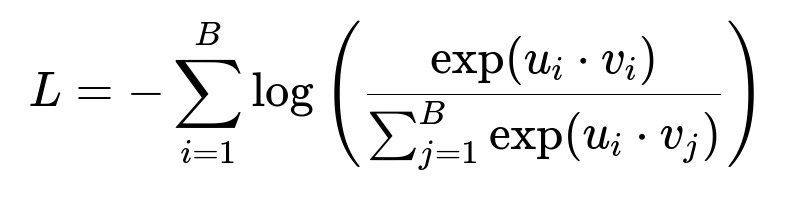
i indexes the query examples in the batch. j indexes the candidate items in the batch. u_i dot v_i is the dot product for the positive pair. u_i dot v_j is the dot product for the i-th query and j-th candidate. B is the mini-batch size. The denominator is the sum of exponentiated dot products for all other items in the batch.
logQ correction
logQ correction subtracts log of the candidate’s empirical probability from the logits. Without it, the model is biased toward popular items, as negative samples only come from observed items. This correction factor is crucial to boost recall for less frequent items. The model calculates sampling probability for each item and adjusts logits accordingly.
Implementation details
TensorFlow plus a library like tf-recommenders is common for building the two-tower architecture. A typical approach is:
Define a custom model class that inherits from tfrs.Model.
Implement a user tower and item tower. Each tower is a multi-layer perceptron that transforms features into embeddings.
In the training step, pass user and item embeddings to a tfrs.tasks.Retrieval loss object that automatically computes the in-batch sampled softmax. Enable removal of accidental hits if needed.
Log probabilities for items in the batch if you want to apply logQ. Subtract that from logits.
PySpark helps shuffle data at scale and export it to TFRecords. Simple code snippet:
train \
    .write.format("tfrecords") \
    .option("recordType", "SequenceExample") \
    .option("codec", "org.apache.hadoop.io.compress.GzipCodec") \
    .mode("overwrite") \
    .save(tfrecords_path)
This code block saves your processed data for TensorFlow ingestion. After data is in TFRecords, build a tf.data pipeline for training.
Approximate nearest neighbor
Indexing item embeddings with an ANN library such as ScaNN or FAISS speeds up retrieval. Store the precomputed item embeddings and at inference time compute a single user embedding, query the ANN index, and quickly get top matches.
Evaluation
Main metric is recall@k, capturing how often the relevant item is in the retrieved set. A typical offline approach:
Split data by time (train on earlier periods, test on later).
For each user query in the test set, compute user embedding, get top k candidates from the index, check if the user’s clicked item is in that set.
Summarize recall@k across queries.
logQ correction, output normalization, and feature-engineered embeddings can show large gains in recall. If desired, an additional ranking model can rerank the top candidates.
Training tips
Scaling to large corpora requires careful memory handling. The in-batch negative sampling technique provides efficient training. Another negative sampling refinement is mixing random negatives (unseen items) to ensure coverage. Monitor training with standard TensorFlow features or custom loops, evaluate at intervals by indexing items and measuring recall on a validation set.
Follow-up Question: How does logQ correction work and why is it necessary?
Answer In-batch negative sampling draws negatives from the observed interactions of other items in the same batch. Common items appear more frequently, introducing a popularity bias. logQ correction subtracts the log of the candidate’s sampling probability from the logits, forcing the model to downweight frequently observed items. This effect rebalances training so the model can retrieve less-popular items more accurately. Without logQ, the model might rank frequent items too high. The correction factor is computed by counting the frequency of each item in the training set. Dividing by total interactions yields the probability for that item. The model retrieves that probability from a lookup table and subtracts log(probability) from the dot product logits at training time.
Follow-up Question: Why use approximate nearest neighbor search for retrieval?
Answer Handling millions of items calls for a fast retrieval mechanism. A naive approach computing user dot product with every item is slow (O(N) for N items). ANN indexing reduces retrieval to roughly O(log N) or even constant time in practice. Libraries like ScaNN or FAISS compress and organize item embeddings into data structures that allow quick queries. At inference, the user tower outputs an embedding. Then the system searches this embedding in the ANN index to retrieve a small subset of items that have the highest similarity scores. This is the candidate stage, which can be done in real time.
Follow-up Question: How would you incorporate features beyond static categorical or numerical data?
Answer The two tower framework can accept textual, image, or sequence-based features. For instance, property descriptions can be embedded with a text encoder (e.g., a CNN or transformer layer). Concatenate or combine that embedding with other numerical or categorical features inside the tower. Similarly, to model a user’s historical browsing behavior, feed user interaction sequences into an RNN or transformer sub-layer in the user tower. The final tower output is still D-dimensional and must match the item tower dimension for the dot product.
Follow-up Question: How do you detect and address accidental hits during in-batch negative sampling?
Answer Accidental hits occur if multiple examples for the same item appear in the same batch, making the model incorrectly treat true positives as negatives. One fix is zeroing out logits for identical item ids in the batch. Another approach is creating a mask so the model does not penalize those pairs. The code typically looks for matching item ids and subtracts a large constant from the logits or sets them to negative infinity. Removing these hits ensures that an item’s presence in another example does not confuse the model.
Follow-up Question: How do you handle training efficiency and memory constraints with large item catalogs?
Answer In-batch negative sampling keeps memory usage reasonable by only dealing with mini-batch items. Also, hierarchical embeddings or partitioning strategies can reduce the dimension of lookups. Sharding embeddings or storing them on disk is another approach. Minimizing overhead in data pipelines is crucial. A well-tuned tf.data pipeline that caches, prefetches, and shuffles data can help. For production, it is common to freeze the item tower after training and load item embeddings into an ANN service. The user tower is the only tower evaluated at runtime.