
ML Case-study Interview Question: Forecasting Sales vs. Demand with Global LSTM Time Series Models

Browse all the ML Case-Studies here.
Case-Study question
A large online marketplace wants to forecast both weekly sales and demand for items sold by first-party sellers. Sales are actual purchased units in a week, constrained by available stock. Demand is the hypothetical sales volume if there had been unlimited stock. The marketplace wants forecasts for the next 12 weeks for each item across multiple countries. How would you build a forecasting solution that generates two separate projections (one for sales, one for demand), and how would you handle challenges like limited historical data, intermittent sales, and special events?
Detailed Solution
Modeling Approach
A Global Time Series (GTS) model can handle many time series simultaneously. Each item is treated as part of a large, shared model instead of having a specialized model per item. Research shows that Long Short-Term Memory (LSTM) neural networks or certain tree-based models tend to perform better in GTS settings, but the one-shot multi-step prediction of an LSTM is convenient when predicting several future weeks.
Data Preparation
Some items were introduced only recently, creating short and sparse time series. Items also differ in volume (some have large sales, others almost none), making raw values hard to model. A simple method is to apply a log transform to the sales data to reduce extreme spikes:
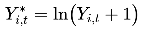
where Y_{i,t} is the sales of item i in week t, and Y_{i,t}^{} is the transformed value. The model then uses Y_{i,t}^{} from previous time steps, along with related features (item visits, questions asked, price changes, stock, etc.).
Sales vs. Demand
Demand differs from sales whenever sales hit the stock limit. If N_{i,t} is the available stock in week t for item i, then the observed sales Y_{i,t} reflect true demand only if:
If:
the true demand might be higher, but it is unobserved. A separate dataset is created where Y_{i,t} is accepted as demand only if it did not saturate stock. A second model then uses that subset for training. Features can include historical sales volumes, online visits, pricing factors, and other signals that might indicate potential sales.
Multi-step Forecasting Details
An LSTM can project the next 12 weekly points at once. For the sales model, historical stock levels help detect items that might be running out. For the demand model, discount information and historic sales patterns help gauge full potential. Both sets of features train independently. At inference, the two models produce separate forecasts: one constrained by expected stock behavior, the other unconstrained.
Handling Zero-Sales Items
If an item had zero sales in recent weeks and was out of stock, the sales model may project near-zero future sales. However, the demand model might predict a recovery if the item becomes restocked. This difference highlights that the sales forecast is the realistic scenario with stock constraints, while the demand forecast is a hypothetical scenario with no constraints.
Performance Evaluation
Metrics like Mean Absolute Error (MAE) avoid complications when the target can be zero. MAE conveys the average deviation in units sold, making it easy to interpret. Other scale-free metrics (like MASE or sMAPE) can be considered, but short time series with many zeros often complicate them.
Special Event Adjustments
Promotions or seasonal events can shift item behavior. Explicitly modeling such events can require custom features and post-processing rules. Sometimes separate event-specific adjustments (e.g., factoring in marketing campaigns) prevent overly complicated training for each country.
Example Code Snippet
A typical LSTM training pipeline in Python might look like this:
import torch
import torch.nn as nn
import numpy as np

class LSTMForecaster(nn.Module):
    def __init__(self, input_dim, hidden_dim, output_dim):
        super().__init__()
        self.lstm = nn.LSTM(input_dim, hidden_dim, batch_first=True)
        self.fc = nn.Linear(hidden_dim, output_dim)

    def forward(self, x):
        lstm_out, _ = self.lstm(x)
        return self.fc(lstm_out[:, -1, :])

# Suppose X_train, y_train are your sequences for many items
model = LSTMForecaster(input_dim=10, hidden_dim=64, output_dim=12)
criterion = nn.MSELoss()
optimizer = torch.optim.Adam(model.parameters(), lr=1e-3)

for epoch in range(50):
    model.train()
    optimizer.zero_grad()
    output = model(X_train)
    loss = criterion(output, y_train)
    loss.backward()
    optimizer.step()
This is a simplified illustration. The actual pipeline would have separate data transformations (including log transforms and stock-based filtering), two distinct training sets (one for sales, one for demand), and more elaborate architecture or hyperparameter tuning.
Follow-up Question 1
How would you handle items that have extremely intermittent demand, such as selling only a few units spread across many weeks?
Answer:
For highly intermittent series, the model may fail to learn reliable patterns because many target values remain zero for most historical time steps. One strategy is to track additional signals beyond historical sales, such as user visits or search queries. These signals may reveal underlying interest even when purchases do not occur. Another approach involves applying specialized transformations that highlight non-zero occurrences. Sometimes separate models for intermittent items help, especially if the main model performs poorly on them. Alternatively, zero-inflation or threshold-based rules can refine forecasts when the model sees extended zero stretches.
Follow-up Question 2
How do you incorporate newly introduced items with extremely short histories?
Answer:
A GTS model pools data from many items, helping it generalize for items with short history. Categorical embedding of product attributes (category, brand, etc.) can supply relevant signals. The model can leverage insights from similar items to predict new items’ performance. If the newly introduced items lack any sales but have visits or user interaction, these features guide the model. If no direct data exists at all, a fallback or cold-start method (using average category-level sales or a nearest-neighbor item) initializes the forecast.
Follow-up Question 3
How would you estimate uncertainty or build probabilistic forecasts for deciding restocks?
Answer:
Generating point forecasts alone ignores the margin of error that is key to inventory decisions. One approach is to leverage Monte Carlo Dropout in neural networks, where dropout is retained at inference, sampling multiple forward passes. Statistical methods such as estimating a suitable probability distribution’s parameters at each forecast horizon can also be used. This yields a confidence interval (or full distribution). These intervals help supply chain decisions under stock constraints by revealing worst-case or best-case scenarios over the next 12 weeks.
Follow-up Question 4
How do you handle large promotions or major external events that do not occur regularly and might not be fully captured by the training data?
Answer:
A typical solution is to apply a post-processing step. If a future large promotion is scheduled, an event-based adjustment can shift the base forecast. The shift might be derived from historical promotion lifts of similar items. For brand-new types of promotions, the adjustments can rely on broader historical analogies or external signals. Maintaining a modular forecast pipeline (model first, event correction second) keeps training simpler and avoids forcing the model to memorize rare spikes.
Follow-up Question 5
How would you validate the effectiveness of your final forecasts before full deployment?
Answer:
Model validation includes rolling time-window backtests, where you retrain on earlier data and predict a subsequent block of weeks. This simulates real production conditions. Additional offline experimentation checks how well the forecasts inform real restocking decisions or cost-saving measures. Online A/B testing compares the new forecast-driven strategy with existing processes. If outcomes like stock outages or overstocking reduce, it validates the forecasting approach.
Follow-up Question 6
Explain the advantage of using MAE over MAPE or MASE in your scenario.
Answer:
MAE is a direct measure of unit-based deviation, so it handles weeks with zero sales smoothly. MAPE and MASE can break down or become undefined if many zero values appear. MASE also assumes each time series is sufficiently long to calculate the Naïve Forecast error for scaling. In short-horizon, sparse retail datasets, MAE gives a clear average error in the same units as sales, ensuring consistent evaluation across items with zero or small volumes.