ML Case-study Interview Question: Automated Observational Causal Inference Platform for Measuring Treatment Effects at Scale.

Browse all the ML Case-Studies here.

Case-Study question

You are tasked with designing and implementing a large-scale observational causal inference platform for a social networking product with hundreds of millions of users. The product team needs to measure how certain non-randomized “treatments” (such as exposure to marketing, infrastructure outages, policy changes, and so on) impact key business metrics. Traditional A/B experimentation at the user level is impossible for some of these cases. Your role is to architect a solution that enables any data scientist on the team to run robust observational causal studies quickly, without deep coding efforts, and to ensure the results are accurate enough to guide product decisions. Describe how you would design and build such a platform, what methods you would include, how you would handle confounding and data pipelines, and how you would ensure the final estimates are trustworthy.

Proposed Solution

Overview of the Platform

A central platform can provide a user-friendly interface to set up the causal study configuration, specify which metrics will be used as outcomes, define control or treatment cohorts, and select relevant confounders. A web application layer can guide data scientists step-by-step and automatically create the data pipelines in the backend. All the heavy lifting of data joins, date alignment, feature extraction, and model runs must happen behind the scenes, so that domain experts only specify what they need, rather than manually coding data transformations.

Data Preparation and Configuration

Accurate causal inference requires carefully timed data. Covariates (predictive variables) must come from a period preceding the exposure or treatment, while the outcome metric must be measured after the treatment is administered. A typical fixed effect model for panel data often involves multiple time periods. Handling these time periods manually is error-prone. A reliable platform automates the extraction of covariates over the correct date windows, merges them with the correct treatment indicators, and aligns the outcome metrics so that they appear strictly after the treatment window.

Scalable data processing jobs could run on Apache Spark clusters, augmented by Java or R components as needed. The system can also integrate with a feature store that maps a human-readable confounder name into a specific data source and aggregation. This standardization avoids repeated ad-hoc data engineering across teams. When a user selects variables such as “7-day session count,” the platform automatically applies the correct joins and time filters to produce the final modeling dataset.

Observational Causal Methods

Different methods suit different contexts. Cross-sectional data might employ matching approaches or doubly robust (DR) estimators. With repeated measurements per unit over time, fixed effects models can remove time-invariant confounders. When an external instrument exists, one might use instrumental variables (IV). For purely time-series interventions at an aggregate level, Bayesian Structural Time Series (BSTS) can handle pre/post trends. A robust platform typically offers these methods:

1. Coarsened Exact Matching (CEM).

2. Doubly Robust Estimator (also called Augmented Inverse Propensity Weighting).

3. Instrumental Variables (IV) Estimation.

4. Fixed Effects Models (FEM) for panel data.

5. Bayesian Structural Time Series (BSTS) for aggregated time series.

Doubly Robust Estimator Example

One of the popular cross-sectional methods is the DR estimator. It combines a regression model for the outcome and a model for the probability of treatment. In its simplest form:

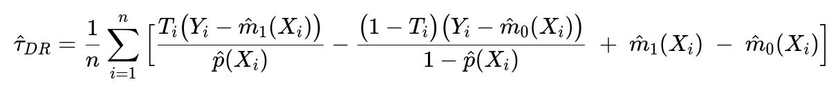
T_i is the observed treatment (1 if treated, 0 if not), Y_i is the outcome, X_i is the vector of covariates, p-hat(X_i) is the estimated propensity to receive the treatment, and m-hat_1(X_i), m-hat_0(X_i) are predictions from outcome models under treatment and control, respectively. The first fraction re-weights the outcome by the inverse of the estimated propensity score, while the second fraction adjusts for outcome regressions. If either the propensity or outcome model is correct, the estimate remains unbiased, hence “doubly robust.”

Automation of Robustness Checks

Robustness checks are essential. An “A/A” test is where the same “treatment” is assigned to both groups so the causal effect should be zero. If the estimated effect is significantly non-zero, that indicates residual confounding, selection bias, or other problems. The platform can automatically run such checks with every analysis. If these checks fail, no one can claim causal findings from that study.

Another possible check is a randomization inference test for cases where partial randomization might exist. One can repeatedly shuffle the treatment and verify that the average treatment effect distribution remains centered around zero if no real treatment effect is present.

Review and Iteration

A formal committee review ensures correct study design and interpretation. The team might verify the user’s choice of confounders, time windows, and whether assumptions for methods like IV or BSTS are reasonable. All past study versions, including code logs, should be tracked to avoid p-hacking. This review step is often mandatory before finalizing any product or strategy decision based on the results.

Example Code Snippet for DR Analysis

Below is a hypothetical Python snippet illustrating DR estimation. The snippet assumes you have properly merged the data, trained models for outcome predictions, and estimated propensity scores.

import numpy as np
import pandas as pd

# df contains columns: treatment, outcome, prop_score, mhat_treated, mhat_control

df['inv_prop_weight'] = df['treatment'] / df['prop_score'] - (1 - df['treatment']) / (1 - df['prop_score'])
df['outcome_reg_adj'] = df['mhat_treated'] - df['mhat_control']
df['residual_adj'] = (df['treatment'] * (df['outcome'] - df['mhat_treated'])) / df['prop_score'] \
                     - ((1 - df['treatment']) * (df['outcome'] - df['mhat_control'])) / (1 - df['prop_score'])

df['dr_est'] = df['residual_adj'] + df['outcome_reg_adj']
dr_estimate = np.mean(df['dr_est'])
print("Doubly Robust Estimate:", dr_estimate)

Follow-Up Question 1

Explain how you would handle unobserved confounders in this platform. What additional methodological checks or approaches could reduce bias from variables not captured in the data?

A thorough solution acknowledges that unobserved confounders cannot be directly controlled, so one must consider methods or designs that weaken their impact. Fixed effects models can remove any time-invariant unobserved factors, provided you have panel data with multiple time periods per user. Instrumental variables can handle unobserved confounding if you find a valid instrument that predicts treatment while not affecting the outcome except through the treatment. Synthetic controls or Bayesian Structural Time Series can help in certain aggregated time-series settings, assuming comparable control units or stable pre-treatment trends. Finally, domain knowledge can guide the choice of plausible sensitivity analyses: for instance, run bounding analyses that assume some range of unknown confounders’ effects. Combine these approaches with thorough peer reviews and business insights.

Follow-Up Question 2

Why is it important to keep a thorough record of all study iterations, and how can we avoid p-hacking in observational causal inference?

Logging every iteration ensures transparency. When a data scientist tries different model specifications, covariate sets, or time windows, each change can influence the estimated treatment effect. A system that automatically tracks every configuration prevents researchers from omitting “failed” configurations in pursuit of a significant result. Publicly documenting every run, including failed A/A tests, rejected covariate sets, and negative or non-significant results, curtails selective reporting. Requiring a formal pre-registration or a review committee sign-off before finalizing a result also helps. Rigorous iteration logs and version control make it harder to hide unsuccessful attempts, thus reducing the risk of p-hacking.

Follow-Up Question 3

How do you decide which of the five methods (matching, DR, IV, FEM, BSTS) to select for a given observational study?

It depends on the data structure, the nature of the treatment assignment, and the assumptions you can credibly make:

• If you have cross-sectional data with no strong time component, matching or DR is simpler.

• If you have panel data with multiple time points, fixed effects can remove any time-invariant confounding.

• If you have a valid instrument that affects the outcome only through the treatment, use IV.

• If you must measure the causal impact at an aggregate timeseries level (for instance, a product-wide policy change on a single day), a BSTS approach can fit the pre/post trend. Domain knowledge and the existence (or lack) of certain variables also inform your choice. The platform should guide you through these decision points.

Follow-Up Question 4

Give an example scenario where Bayesian Structured Time Series (BSTS) might be preferred over a fixed effects model, and describe the assumptions BSTS relies on.

BSTS might be better if you have a single aggregated time series (for example, daily signups across the entire platform) before and after a broad external intervention such as a regional policy change. A fixed effects approach usually requires multiple cross-sectional units observed over time. BSTS relies on the assumption that past trends for a control or counterfactual can predict the trajectory of your outcome in the absence of intervention. You typically need a period long enough to capture major seasonal patterns. BSTS also assumes that the post-treatment outcome can be compared to a synthetic forecast generated from historical data before the treatment. If the forecast diverges significantly from actual observations, that difference is interpreted as the treatment effect.

Follow-Up Question 5

Why is randomization (as in classic A/B experiments) still considered the gold standard, and what would motivate you to use an observational approach even when randomization is possible in principle?

Randomization eliminates systematic differences between treatment and control groups except for the treatment itself. Observational methods must statistically remove imbalances, but they cannot address unobserved variables that were never measured. Randomization is straightforward and less assumption-dependent. However, there are many real-world scenarios where randomization is too costly, infeasible, or unethical. These scenarios include large-scale marketing campaigns with no user-level randomization, or significant infrastructure downtime that cannot be assigned randomly. Observational approaches fill this gap, letting researchers estimate causal effects when they simply cannot run a standard experiment.

---