
ML Case-study Interview Question: Balancing Relevance and Diversity in Recommendations via MMR Re-ranking

Browse all the ML Case-Studies here.
Case-Study question
A major online travel company wants to increase the variety of its accommodation recommendations. They have a baseline popularity-based model that provides top-ranked items by predicted relevance. They notice low user engagement when recommendations are too homogeneous. They have numerical features (like price and review count), categorical features (like star rating), and multi-valued features (like amenities) to represent each property. They also have an optional learned embedding model. They want to implement a strategy that balances relevance (ranking metrics such as Normalized Discounted Cumulative Gain) with diversity (average dissimilarity among recommended items). How would you design a solution to inject diversity into their final recommendation output? Outline a feasible approach, discuss the key algorithms, and suggest how you would balance diversity against relevance.
Proposed Detailed Solution
Combining a scoring model with a post-processing re-ranking step is effective for introducing diversity without requiring complex changes to each individual model. Multiple methods can be used:
Clustering-based re-ranking
Neighborhood Cosine Distance approach (also known as Maximal Marginal Relevance)
Each method has tradeoffs regarding explainability, user relevance, and implementation complexity.
Short explanations follow:
Clustering approach Re-rank by selecting items from different clusters. Properties grouped together are assumed similar, so pulling items from distinct clusters increases variety. If clustering uses explicit features (like amenities or price buckets), balancing these features leads to more controlled diversity. A drawback is lowered ranking metrics if many clusters have lower-relevance items.
Neighborhood Cosine Distance (MMR) approach Compute a new score that accounts for both item relevance and similarity to already-selected items. A higher diversity weight focuses more on dissimilarity. A lower diversity weight focuses more on traditional relevance.

Where:
relevance(item) is the original model’s score.
similarity(item, selected) is the maximum similarity between the item and any already-selected item.
alpha is the diversity weight. Closer to 1 puts more emphasis on dissimilarity.
Intralist Dissimilarity Metric A typical way to track diversity in a recommendation list is to compute the average pairwise distance among recommended items:
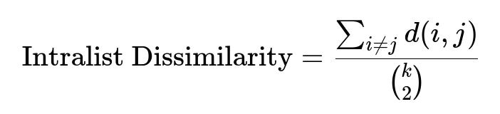
Where:
d(i,j) is a distance measure (like Euclidean or 1 - cosine_similarity).
k is the number of recommended items in the list.
The summation is over all distinct pairs.
Larger values indicate higher variety. Scaling or transforming numerical features (e.g., log transform for skewed distributions) and one-hot encoding for categorical features keep comparisons fair when computing similarity.
Implementation steps:
Score items using the baseline ranking model.
Construct item embeddings either from explicit features (price, star rating, amenities, etc.) or from a learned representation.
Apply a re-ranking step:
For clustering: assign each item to a cluster. Reorder the top items by ensuring picks from different clusters.
For MMR: pick the top item by relevance, then iteratively add items that have the highest MMR score.
Tune the diversity weight alpha or number of clusters. Observe how Normalized Discounted Cumulative Gain changes with intralist dissimilarity.
Code snippet for intralist dissimilarity (Python-like pseudocode):
def intralist_dissimilarity(embeddings, predictions, k=10):
    order = np.argsort(predictions)[::-1][:k]
    top_embeddings = embeddings[order]
    pairwise_dists = cdist(top_embeddings, top_embeddings, metric='euclidean')
    sum_of_dists = pairwise_dists.sum() / 2
    comb = k * (k - 1) / 2
    avg_dist = sum_of_dists / comb
    return avg_dist
Explanation:
embeddingsis an array of shape (num_items, dimension).predictionsis the relevance score vector.kis how many top items to evaluate.cdist(...,'euclidean')computes pairwise distances among items.Summation of the upper or lower triangle is divided by the number of pairs for the average distance.
Tuning:
A higher diversity weight alpha in MMR picks more varied items but may reduce ranking performance.
A balanced approach improves user satisfaction by exposing them to properties spanning different price buckets, amenities, and star ratings.
Follow-Up Question 1
How would you handle a situation where increasing diversity decreases Normalized Discounted Cumulative Gain too much?
Answer Test small increments in the diversity weight alpha or cluster-based selection fraction. Evaluate offline metrics to find a sweet spot on the diversity-relevance tradeoff curve. Check user feedback or A/B test in production to confirm. If ranking metrics decline severely, limit how many items get replaced during the re-ranking. Another option is dynamic tuning of alpha based on user context. For instance, if a user is extremely price sensitive, reduce alpha to keep top results relevant to price. If a user is exploring, increase alpha.
Follow-Up Question 2
What if some features or embeddings are outdated or missing for certain items?
Answer Fallback to partial similarity. Use available features (like star rating or partial embeddings) when full data is missing. If certain features are noisy or stale, remove them from re-ranking. For a learned embedding approach, periodically retrain embeddings on fresh logs or maintain an incremental update pipeline. Missing data can also be imputed by average or median values before computing pairwise distances, but do that cautiously and evaluate if it hurts the reliability of the distance measure.
Follow-Up Question 3
Explain how you might adjust your method when users demand more transparency in why they see recommendations.
Answer Use explicit feature-based diversity. Show how items differ by star rating, amenities, or price range. Provide a brief message: “We’ve included budget-friendly and luxury options” for clarity. If a learned embedding is used, highlight interpretable aspects of the item: “This hotel is recommended for its central location and unique amenities.” Avoid black-box approaches if explaining the property differences is a priority.
Follow-Up Question 4
How would you efficiently scale the Neighborhood Cosine Distance re-ranking step for millions of items?
Answer Restrict re-ranking to the top N items from the baseline model. Then apply the MMR formula on that subset. Caching or approximate nearest neighbor techniques help manage similarity computations for large embeddings. Parallelize distance calculations using vectorized libraries (e.g., NumPy or GPU operations). For distributed environments, split item embeddings across workers and gather partial results. Also consider sampling or partial-scan heuristics if real-time latency is crucial.
Follow-Up Question 5
Why might clustering on learned embeddings sometimes lead to poor results for real-world ranking tasks?
Answer Neural embeddings can place popular items close together, skewing cluster sizes. Some clusters might have mostly niche items that are rarely viewed or transacted, hurting ranking if forced into the top recommendations. Explaining cluster assignments is harder when embeddings encapsulate many abstract factors. Data biases and insufficient coverage of less popular items can produce clusters lacking strong signals. For real-world tasks, carefully test whether the embedding-based clusters align with user preferences.
Follow-Up Question 6
How would you detect if your re-ranking method introduces unintended biases?
Answer Continuously track metrics that matter for fairness or coverage. For geographic bias, confirm if your re-ranked results over-represent certain locations. For amenity bias, see if certain amenity categories never appear. Conduct offline checks with user demographic data when appropriate. If discovered, add constraints or weighting schemes that enforce coverage targets. For instance, ensure each region has at least one recommended property or each star rating is represented.
Follow-Up Question 7
Could you mix explicit and learned embeddings for diversity?
Answer Yes, by concatenating or weighting them in a joint vector or by combining two distance functions. For instance, half the time measure the distance from explicit features, and half the time from the learned embedding. This adds interpretability while still capturing hidden relationships. Tuning how much weight to place on each is key, so run experiments or A/B tests.
Follow-Up Question 8
What is the advantage of post-processing re-ranking over embedding-level changes to the model?
Answer No need to retrain the core model. Re-ranking can be layered on existing pipelines. Switching or adjusting diversity features is simpler. If multiple recommendation models exist, the same re-ranking logic can serve them all. Embedding-level changes require specialized training steps, more complex hyperparameter tuning, and deeper infrastructure modifications. Post-processing is more flexible for quick iteration.
Follow-Up Question 9
What techniques would you use to handle high-cardinality or multi-valued categorical features like “amenities” in the distance metric?
Answer Apply multi-hot or one-hot encoding. Convert each amenity into a binary flag. Weighted or Jaccard distances can help if you care about coverage of distinct sets. If certain amenities matter more, weight those features higher in the distance measure. For memory efficiency, consider sparse representations. For large amenity vocabularies, run dimensionality reduction or specialized embedding for amenity sets, then incorporate that embedding in the final item vector.
Follow-Up Question 10
Provide an example of code logic to implement MMR re-ranking with a relevance score array and explicit embeddings.
Answer
def mmr_rerank(items, relevance_scores, embeddings, alpha, k):
    selected_indices = []
    candidate_indices = list(range(len(items)))
    # Pick the top item by relevance first
    best_index = np.argmax(relevance_scores)
    selected_indices.append(best_index)
    candidate_indices.remove(best_index)

    while len(selected_indices) < k and candidate_indices:
        best_candidate = None
        best_mmr_score = -9999
        for idx in candidate_indices:
            rel = relevance_scores[idx]
            # Similarity is negative distance or dot product
            sim_to_selected = max(
                1 - cosine(embeddings[idx], embeddings[s])
                for s in selected_indices
            )
            mmr_score = alpha * rel - (1 - alpha) * sim_to_selected
            if mmr_score > best_mmr_score:
                best_mmr_score = mmr_score
                best_candidate = idx
        selected_indices.append(best_candidate)
        candidate_indices.remove(best_candidate)

    return [items[i] for i in selected_indices]
Explanation:
itemsis a list of item IDs.relevance_scoresis an array of the initial model’s predictions.embeddingsis a 2D array of explicit or learned vectors.alphais the diversity weight.Repeatedly select items with the highest combined relevance and distance from already-chosen items.