ML Case-study Interview Question: Classifying Intersection Controls using CNNs on Telemetry-Derived Speed Images

Browse all the ML Case-Studies here.

Case-Study question

A ride-hailing organization needs a reliable way to detect stop signs and traffic signals at intersections across multiple cities. The data consists of anonymized driver telemetry (speed, GPS traces) collected from drivers approaching various intersections. The goal is to accurately classify each intersection as having a stop sign, a traffic signal, or neither. Propose a complete end-to-end machine learning pipeline to perform these classifications. Explain how you would gather the data, label the data, design the model, train it, evaluate performance, and ensure scalability and generalization to new regions. Assume large volumes of noisy sensor data and potential GPS inaccuracies. Prepare to handle corner cases such as multi-segment intersections and variable driving patterns.

Most Detailed In-Depth Solution

Overall Approach

Use driver speed and location readings to identify distinct velocity patterns near intersections. Transform these data points into images or structured representations. Train a convolutional neural network to classify each intersection’s traffic control type: stop sign, traffic signal, or neither.

Data Acquisition and Preprocessing

Gather driver telemetry with timestamps, speed, GPS position, and bearing from a wide timeframe. Filter for high GPS accuracy. Align each trace to the correct intersection approach by matching the bearing of the road segment with the bearing of the vehicle. Normalize samples to reduce skew from different vehicle types or traffic volumes.

Intersection Bounding Boxes

Construct bounding boxes around intersections by examining where roads meet. Keep those with up to four road segments to simplify classification. If two bounding boxes overlap, reduce overlap to ensure each intersection is isolated. This preserves consistency when labeling.

Labeling

Match each bounding box to known traffic control elements. If an intersection has a stop sign, label it accordingly. If it has a traffic signal, label it as such. Otherwise, label it as neither. Use official city or publicly available traffic sign inventories where possible.

Kernel Density Estimation

Aggregate speed-distance points within each bounding box to capture velocity profiles as drivers approach. Apply a 2D kernel density estimator with a Gaussian kernel. Convert the resulting densities into images showing how speed changes with distance from the intersection.

Neural Network Classifier

Feed these images into a pretrained convolutional neural network (such as a variant of VGG). Initialize with ImageNet weights and fine-tune all layers to classify the images into three classes. Use an additional fully connected layer at the end to output three probabilities.

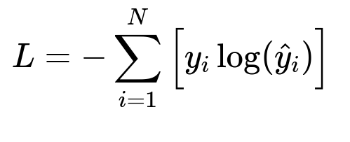
Where y_i represents the true label (one-hot format) and hat{y}_i is the predicted probability for the correct class. N is the batch size.

Training

Perform hyperparameter tuning on the learning rate, batch size, and number of epochs. Monitor training and validation accuracy. Confirm minimal overfitting by checking if training and validation curves stay close.

Evaluating Generalization

Test on a different city with varied proportions of stop signs, traffic signals, and neither. Compare model outputs against ground truth or curated data. If performance remains robust, the model likely generalizes to new regions.

Implementation Example

Train with Python and popular frameworks like TensorFlow or PyTorch. Load telemetry data from a data warehouse. Construct the 2D kernel density images. Convert them to tensors, and feed into the CNN for training. Use a simple script:

import torch
import torch.nn as nn
import torch.optim as optim

model = MyVGGBasedModel()  # Custom extension of a pretrained VGG
criterion = nn.CrossEntropyLoss()
optimizer = optim.Adam(model.parameters(), lr=0.0001)

for epoch in range(num_epochs):
    for images, labels in train_loader:
        optimizer.zero_grad()
        outputs = model(images)
        loss = criterion(outputs, labels)
        loss.backward()
        optimizer.step()

Train for a certain number of epochs until validation accuracy stabilizes. Conduct final testing on unseen data. Evaluate false positives and false negatives and refine filtering thresholds if needed.

Scalability

Distribute the training process by sharding data across multiple nodes or using cloud resources. Use data pipelines that can handle large-scale ingestion of telemetry. Store model artifacts in a versioned repository. Deploy the model as a microservice that can update intersection classifications as new data arrives.

Practical Insights

Clean up noisy signals, especially near high-rise buildings. Calibrate threshold-based confidence to reduce false alarms. Re-run labeling as the map changes. Validate suspicious intersections with ground surveys if needed.

Follow-up question 1: How would you address intersections that have multiple lanes or complex layouts?

Use more granular bounding boxes for each lane or approach segment. Split bounding boxes so each lane is considered separately. For multi-lane or unusual layouts, confirm label consistency. Expand the classifier input to include additional features like average bearing or turning patterns if raw speed data alone is insufficient.

Follow-up question 2: How would you handle intersections where traffic lights sometimes behave like stop signs (for instance, flashing red lights at night)?

Include temporal metadata showing time-of-day or known schedules for traffic light changes. Label certain intersections as traffic signals but incorporate time-dependent patterns if available. Add a subclass for blinking traffic signals and collect training data showing these scenarios.

Follow-up question 3: How would you reduce false positives in regions with heavy congestion where cars frequently stop for reasons other than a traffic sign or traffic signal?

Apply advanced filtering. Exclude long stops caused by traffic jams by comparing stops across multiple days or multiple vehicles. Consistent stopping in the same location across varied times strongly indicates a traffic control element. Isolated stopping patterns at peak hours might be congestion related, so discount them or assign lower classification confidence.

Follow-up question 4: How would you extend this to classify other road signage (yield signs, pedestrian crossings) while preserving performance?

Collect sufficient labeled data for new sign types. Retrain or finetune the existing CNN on a multi-class problem. Separate training sets for new sign categories can help the model learn additional patterns. Ensure robust augmentation to handle data imbalance. Validate performance on each category to detect confusion between similar signs.

Follow-up question 5: How would you integrate map corrections in real-time as telemetry data continues to arrive?

Implement a streaming pipeline. Batch incoming telemetry, update kernel density estimations on a rolling basis, and feed them to the classifier on scheduled intervals. Re-classify intersections that show statistically significant changes in speed patterns. Use version control for these newly inferred labels. Deploy automated checks or partial manual verification for high-risk changes.

Follow-up question 6: How would you handle edge cases such as GPS drift or device sensor errors that produce misleading speed-distance plots?

Filter data points with low GPS confidence. Resample data for consistent intervals. Cross-check driver velocity with inertial sensor data if available. Discard outliers from kernel density inputs, especially if abrupt shifts in location or speed do not match realistic driving patterns. Train a separate anomaly detection model to detect corrupted traces.

Follow-up question 7: How would you adjust your approach for a more rural environment with fewer intersections or different driving habits?

Lower the bounding box threshold for intersection coverage because roads may be less dense. Adjust the classifier’s thresholds to accommodate higher speeds. Gather more data over time because rural roads may have fewer examples of stop-and-go patterns. Maintain the same core CNN architecture but be prepared to refine kernel bandwidth parameters or add new features if driver behavior differs significantly.

Follow-up question 8: How would you evaluate whether using a simpler traditional machine learning approach (like random forests) might suffice?

Compare performance against a baseline random forest or other methods trained on engineered features (stop frequency, average stop duration). Benchmark classification metrics on holdout sets from multiple cities. If a simpler method achieves close accuracy with less computation, weigh its efficiency and interpretability against the CNN approach. If the gap is large, the CNN approach is preferable.

Follow-up question 9: How would you ensure the model remains robust over time as traffic behaviors evolve?

Schedule periodic re-training. Continuously sample new telemetry. Update the training set to reflect seasonal or infrastructural changes. Monitor metrics in production. Trigger partial re-labeling if performance drops on real-world data. Retrain the CNN on combined old and new data for stable, continuous improvement.

---