
ML Case-study Interview Question: Accurate Two-Wheeler Distance Prediction via ML and Synthesized Ground Truth

Browse all the ML Case-Studies here.
Case-Study question
You are tasked with building a real-time system that predicts point-to-point two-wheeler travel distance in a high-volume delivery environment. Existing map providers offer noisy or incomplete two-wheeler distance estimates. Your historical data includes GPS trajectories from riders, and also multiple additional distance estimates: haversine distance, OpenStreetMap (OSM)-based GraphHopper distance, and snapped route distance. These sources often conflict with each other due to missing road segments, map errors, or GPS noise. The goal is to create an accurate two-wheeler distance prediction model that scales to production-level volumes and adapts to changing road conditions. How will you design, implement, and deploy a machine learning model that uses various noisy distance estimates and spatio-temporal features to predict two-wheeler travel distance?
Address the following:
Straight away explain how you will obtain reliable ground truth travel distances from noisy sources. Explain your feature engineering approach. Discuss the model architecture, handling sparse data, and fallback strategies. Show how you monitor error metrics in production and continuously improve predictions. Propose a mechanism for error masking if certain regions or road networks go stale or inaccurate. Explain your approach to ensuring stable performance during major disruptions, such as road closures or lockdowns.
Detailed solution
Background
Accurate point-to-point two-wheeler distance predictions require reliance on multiple sources: GPS trajectories, OSM-based routes, and approximate calculations like haversine. Each source has noise. A robust synthesis is needed to obtain a final ground truth. Historical trip data, aggregated over specific regions and time periods, also strengthens model inputs.
Y-label Synthesis (Ground Truth Creation)
Reliable labels are derived by merging all available distance estimates. Each trip has various distance values: trajectory distance, snapped route distance, OSM distance, and potentially more. Each value can be off for different reasons. A matching strategy groups matching distance estimates (within a small threshold) into equivalence classes. The final label becomes the smallest average among any non-singleton equivalence classes.
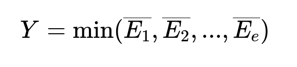
Here:
S = [Y1, Y2, ..., Yv] is the set of distance estimates from v sources.
E1, E2, ..., Ee are the non-singleton equivalence classes.
Each overline{E_k} is the average of all distance estimates in class E_k.
Y is chosen as the minimum average among those equivalence classes.
This approach ensures the final label is consistent across at least two diverse sources. If all distances differ by more than a small threshold, the model discards that trip (no ground truth label).
Feature Engineering
Design real-time and historical features that capture distance patterns:
Real-time features: Haversine distance between start and end points. OSM-based distance for the same route. Time-of-day indicators (peak vs off-peak hours).
Historical features: Distances aggregated over geohash pairs at levels L8 or L7. Aggregations at different time windows (7-day, 60-day) to adapt to temporal fluctuations. Slot-based grouping for traffic patterns.
Source confidence: OSM Trip Count for how often OSM distance matched the final ground truth in that geohash pair. If OSM is usually right in a region, the model relies on it more.
Model
A non-linear regression model (random forest or gradient boosted trees) handles the interplay among real-time distance estimates and historical features. Deep learning can be used, but a tree-based method often performs well with tabular data. Large distances or rarely traveled routes have low coverage, so the system falls back to a simpler distance estimation approach when data are sparse.
Handling Sparse Data
Some start-end geohash pairs have little historical volume. The model with inadequate training data in these areas defaults to the fallback system. This yields high coverage while preserving accuracy for well-traveled routes.
Monitoring and Feedback Loop
Check real-time errors by comparing predicted distances to newly obtained ground truth from fresh trips. Persistently high error in a region triggers masking. If a geohash pair or route path shows large variance, predictions are ignored for that pair. Once new historical data stabilizes, the system demasks that region.
Adapting to Disruptions
Sudden closures or lockdowns alter routes. Using rolling time windows (7-day, 60-day) and continuous data ingestion helps the model learn new paths. Fallback rules remain for severely disrupted roads. Masking ensures major changes do not degrade overall performance.
Code Example
import pandas as pd
from sklearn.ensemble import RandomForestRegressor

# Suppose df has columns:
# haversine_dist, osm_dist, historical_avg_dist_7d,
# historical_avg_dist_60d, osm_trip_count, time_slot, synthesized_dist

# Features and labels
X = df.drop(columns=['synthesized_dist'])
y = df['synthesized_dist']

model = RandomForestRegressor(n_estimators=100, max_depth=12, random_state=42)
model.fit(X, y)

# Prediction
predictions = model.predict(X)
Explaining in simple terms: The training pipeline merges multiple distance estimates and compiles them into a final ground truth. Then the pipeline builds features reflecting real-time data (haversine, OSM) plus aggregated features over geohash/time. A random forest predicts final distance at request time. A feedback loop monitors performance, applying error masking as needed.
What if you only had OSM distance and no other distance sources?
A single distance source without GPS or other providers is more prone to errors. The ground truth generation step would be limited. A potential fix is collecting more data from actual trips to refine or override OSM predictions. The historical feature base would grow once enough real trips are gathered. Temporary short-term solutions might rely on standard fallback heuristics.
How do you select the threshold for equivalence classes?
A small threshold (like 100 m) ensures the two distances are probably for the same route. A narrower threshold can exclude real matches if GPS noise is high. A larger threshold risks grouping unrelated distances. Calibrate it by analyzing typical route distance variance.
How do you maintain speed when distance requests are extremely high in production?
Pre-compute aggregated features at geohash pairs. Load a trained model in a fast inference service (e.g., a microservice with minimal overhead). Use caching to quickly retrieve repeated requests for frequent routes. The final step is a lightweight model predict call.
What is your approach when you spot large errors in a few high-volume corridors?
Mask those corridors automatically if their errors repeatedly exceed a preset limit. The fallback system steps in for them. Once fresh data show stable improvement, remove the mask. This prevents major errors from repeatedly occurring and harming the business metrics.
How do you keep this model robust across large geographic expansions?
Design the pipeline to ingest data from new cities or regions. Let the equivalence-class method adapt quickly whenever at least two distance estimates agree. Use a data-driven approach for any region that accumulates enough real trips to train. Otherwise, keep fallback logic as a universal safety net.
How do you handle completely new routes with no historical data?
Use haversine or OSM distance as a baseline. Mark such routes for immediate data collection. Once some trips occur, incorporate them into the pipeline, synthesize ground truth, and retrain or incrementally update. The real-time system transitions from fallback to model-based predictions once coverage is adequate.
How would you handle a small number of GPS samples per trip?
Sparse GPS sampling can cause inaccurate trajectory distance. Map-matching might be less reliable. Consider improved on-device sampling or interpolation logic. If you cannot improve sampling, weigh that distance source lower unless it aligns closely with other distance providers.
What if your model systematically underestimates or overestimates?
Check error distributions across regions, time slots, and distances. Apply targeted bias corrections or retrain with custom loss functions that penalize large errors. Regularly refresh training data to avoid concept drift and re-validate threshold and mask logic.
How do you validate performance before full rollout?
Compare the model’s distance predictions to newly collected ground truth data for a random subset of trips. Track mean absolute error (MAE) and error distribution. Pilot in limited areas. If performance meets error benchmarks, expand coverage. Log any anomalies for debugging.
Why use random forest or gradient boosted trees instead of a neural network?
Tree-based models often excel with structured data and explicit features. They handle sparse data and missing values well. Neural networks can help if you have huge data volume and more complex feature interactions. However, random forests are simpler to tune and easier to interpret.
What if OSM incorrectly marks one-way roads or missing routes?
OSM-based distances might deviate significantly in certain geohashes. The equivalence class method drops OSM distance if it fails to match other sources. The fallback system remains safe. Over time, if GPS-based or snapped-route data consistently contradicts OSM, that portion of OSM data gets flagged as unreliable.
How do you continuously refine this system?
Collect new trips daily. Run them through map-matching, OSM queries, and distance calculation. Synthesize new ground truth. Retrain or update model weights and error masks. Re-deploy frequently. Monitor real-time performance metrics (MAE, coverage), and investigate outliers.
How do you ensure minimal disruptions to the business while deploying changes?
Use a multi-phase rollout. Shadow-test new predictions alongside current ones in a passive mode. Compare errors. If stable, direct small traffic to the new model. Gradually ramp up coverage. Maintain versioning so you can revert quickly if you see performance drops.