
ML Case-study Interview Question: Long-Term Rideshare Forecasting with Spline-Exponential Cohort Retention Curves.

Browse all the ML Case-Studies here.
Case-Study question
A ridesharing platform wants to forecast driver hours (supply) and ride requests (demand) up to 52 weeks into the future. They track weekly cohorts of new users (either drivers or riders) based on when each user first joined and in which region they joined. Each cohort’s behavior changes over time as some users become inactive (churn) or return (resurrect). They discovered that early weeks for a new cohort do not follow a smooth exponential shape because of user diversity (tourists, promo-seekers, etc.). They also see seasonal effects and region-to-region differences. They are seeking a senior Data Scientist to propose a complete end-to-end system to:
Build or select a model for cohort-based long-term forecasting.
Accommodate situations with few data points for newer cohorts.
Estimate unknown future cohorts.
Handle heterogeneous behaviors during early weeks vs. later weeks within cohorts.
Incorporate parallel computing or other methods to handle large-scale data efficiently.
Explain how you would design this system, estimate its parameters, tune hyper-parameters, and use the results to forecast both supply and demand. Include how you would validate and backtest your model. Outline any strategies to handle missing or partial data for new or immature cohorts.
Provide your end-to-end approach from data ingestion, modeling, validation, to final deployment in production.
Detailed solution
Overview of the forecasting approach
A combination of exponential-like retention curves plus Spline segments can capture how new cohorts behave differently in early weeks. Segmenting cohorts by the week they join in each region allows separate curve fitting for each cohort. In early weeks, user activity can drop fast due to short-term usage or promotional incentives. Later, the behavior becomes smoother and closer to a stable exponential-like pattern.
Retention curve
Active user count (or usage) in a cohort often follows an exponential decay plus a resurrection term. Let y(t) be the total active usage at time t for a given cohort. lambda > 0 is the churn rate, and mu > 0 is the resurrection rate. y(0) is the initial usage at inception.
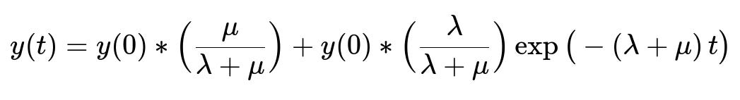
Here, y(0) is the active usage at the start of the cohort’s tracking. t is the week index (or some discrete time unit). lambda is how quickly users leave the platform. mu is how quickly inactive users return. This form ensures a positive steady-state usage at t going to infinity if mu > 0.
Heterogeneity in early weeks
Exponential fits alone often fail in the first few weeks because of different user sub-types. A cubic polynomial or another function can handle this early pattern. A Spline approach connects that polynomial segment to the exponential segment at a knot (such as t = 5 or t = 8) with continuity in function value and derivatives. That Spline curve is estimated separately for each cohort.
Handling multiple cohorts
Each region and join-week define a separate cohort. Mature cohorts (those observed for enough weeks) have enough data to reliably fit Spline-exponential parameters. Newer cohorts have partial or no data, so the system borrows information from mature cohorts by imputing missing observations. This step uses a regression-based approach where new cohorts inherit the shape and average usage patterns of similar older cohorts, plus a stochastic error term for variability.
Demand and supply integration
Driver hours and ride requests per activation are each modeled using the approach above. Summing over all cohorts gives total demand or supply forecasts for each future week. Seasonal factors can be applied on top of the retention curve. If external knowledge suggests large shifts in user acquisition or market expansions, incorporate them into the forecast of new activations.
Steps to implement
Data ingestion combines weekly cohort definitions, aggregated usage, churned vs. active user counts, and region tags. For each cohort, fit a two-part function: polynomial (early) + exponential (later). Assign hyper-parameters:
Maturity threshold beyond which a cohort is considered “mature.”
Extension threshold controlling how much of the younger cohort’s timeline is imputed.
Noise level for stochastic imputation.
Tune these using backtesting with historical data. Once trained, store each cohort’s parameters. For unseen cohorts, project an average shape from recent cohorts. Multiply by forecasted activations. Sum across cohorts to get final weekly predictions.
Parallelization
Each cohort-level curve fit is small, so they can run in parallel across many cohorts. The final step aggregates them for a global forecast. This procedure scales to thousands of cohorts.
Model validation
Perform multi-step ahead backtests and compare predictions to actual usage from older periods. Use statistical error metrics. Check weekly errors, cumulative errors over 3 to 6 months, and bias. Adjust hyper-parameters to trade off bias vs. variance. Compare simpler pure exponential to the Spline approach. Retain the method with smaller errors in out-of-sample tests.
Deployment
Implement the pipeline to run automatically each week, updating forecasts as new data arrives. Monitor performance. If cohorts systematically diverge from predictions, consider adjusting the imputation method or the polynomial portion.
How would you handle sparse data or partial observations in certain cohorts?
Sparse data arises for very young cohorts or for regions where usage is low. Imputation leverages mature cohort patterns. For each missing weekly data point, generate a synthetic usage from a regression model trained on cohorts with enough data, then inject random noise for realism. Estimate the Spline-exponential parameters using the combination of real and imputed data. This ensures minimal overfitting to the few real points while still preserving some unique signals from the small data.
How do you decide where to place the Spline knot, and how do you ensure smooth continuity?
Place the knot where behavior transitions from early volatility to more stable usage. An empirical approach is to choose a fixed time index (like week 6) that typically marks the end of promotions or trial usage. Enforce continuity constraints at that knot. For a cubic polynomial segment from t=0 to t=knot, connect to an exponential for t>knot by matching function value, first derivative, and second derivative at t=knot. Solving these constraints ensures a smooth final curve, preventing abrupt jumps at the junction.
How do you address seasonality in this model?
Use a separate time-series model (like a seasonal additive factor) or a known weekly seasonality coefficient from historical data. Multiply or add that seasonal factor on top of the baseline retention curve. If ride requests are known to spike in summer, adjust each cohort’s weekly forecast by the factor relevant to that week’s seasonality. Calibration can occur once a stable retention model is found. Combine it with the seasonal pattern derived from separate time-series decomposition.
How do you maintain consistency across regions with different user behaviors?
Group regions by similarity in usage patterns. For a new region lacking mature cohorts, pick the most similar region or cluster of regions to borrow its shape parameters. The system can measure similarity by looking at historical user engagement patterns or user demographics. This alignment ensures no region is left without reference data. Once enough weeks pass, the region’s cohorts become self-sufficient with their own data.
Why not just use a large fixed-effects model instead of fitting each cohort separately?
A large fixed-effects model struggles if certain cohorts have minimal observations. It often forces a single global shape with many dummy variables, which can degrade accuracy when user heterogeneity is high. Cohort-level modeling with partial imputation preserves local differences. Each cohort’s early weeks can differ because of local user promotions, events, or demographics, so a more flexible cohort-specific Spline-exponential model can produce lower long-term errors.
How would you extend this approach for driver supply and rider demand interactions?
Model them separately using the same cohort logic. Summarize driver supply cohorts to forecast total available hours. Summarize rider demand cohorts to forecast total rides requested. The platform’s overall operations may then cross-reference the two predictions. A region with forecasted driver hour shortages might trigger incentives for driver sign-ups. Coupling the supply and demand forecasts can also help refine future activation assumptions: if demand surges, sign-up campaigns might shift as well.
How do you scale it to thousands of cohorts while still delivering results quickly?
Create a parallelized pipeline where each cohort’s Spline-exponential fit is independent. Distribute these jobs across computing resources. Store partial results to speed up retraining if only a few new weeks of data arrive. Streamline big matrix operations by segmenting cohorts by region and summing partial forecasts in an aggregated pass. Keep memory usage manageable by storing only the final parameters for each cohort.
What if new business strategies or external factors are not accounted for in historical data?
Incorporate external forecasts for activations or macro indicators. If marketing campaigns are known to double driver sign-ups, modify the activation forecast input. This approach ensures the model’s core structure (retention curves) remains stable while external changes are captured in the base activation numbers. Maintain a process to revise assumptions if data shows unexpected adoption trends.
Why is a high synergy rate lambda + mu relevant?
A high lambda + mu means the system transitions quickly into its steady-state pattern. If churn or resurrection rates are large, user counts rapidly change. Cohort usage stabilizes faster. If lambda + mu is small, the stabilization is slower. Knowing synergy helps interpret how quickly a cohort’s usage will plateau or fade, which affects capacity planning and cost management.
How can we demonstrate real-world impact of this forecasting approach?
Compare actual vs. predicted usage for driver hours or rides over multiple months. Quantify error reductions vs. a simpler baseline. Show how more stable, accurate forecasts enable better resource allocation, marketing budgets, and strategic decisions. Track metrics like mean absolute percentage error for different time horizons (one week, one month, several months). Publicize consistent reductions in long-range forecast errors to justify the complexity of the Spline-exponential methodology.