
ML Case-study Interview Question: Using Denoising Autoencoders to Impute Real Estate Attributes for Accurate Price Prediction.

Browse all the ML Case-Studies here.
Case-Study question
A real estate aggregator collects home data from multiple sources. Patterns of missing or incorrect attributes (such as missing bedroom counts or implausible lot sizes) disrupt the accuracy of their home price prediction model. The goal is to build an imputation model that recovers missing or erroneous property attributes, then measure the impact of these imputations on the final home value predictions. Assume the aggregator uses a deep learning-based pipeline. Propose your solution strategy, outline the model architecture, detail feature engineering steps, and explain how you would evaluate the new imputation approach's effectiveness on the final home value predictions.
Instructions:
Straight away propose your solution. Mention the technology stack, data sampling and pre-processing ideas, model training methodology, and how you would handle evaluation. Explain it as if you are talking to senior Machine Learning colleagues who want to see clear logic and implementation details.
Detailed Solution
Overview
Imputing missing or incorrect features requires robust methods that handle high-dimensional data, diverse variable types, and non-linear relationships. Undercomplete autoencoders represent a powerful approach because they capture latent patterns in data, handle non-linearities, and can reconstruct or predict values missing from noisy inputs. A denoising autoencoder (DAE) tends to perform well for imputation because it learns to recover original signals from partial corruption.
Data Sampling and Preprocessing
Splitting the full dataset into training and test samples is critical. Drawing one million records for training and a subset for validation and testing is a practical strategy when dealing with a large real estate dataset. Geospatial data often plays a role in home attributes, so creating region-based aggregations (quantiles, mode, or average of relevant features) simplifies high-cardinality categorical variables.
Handling outliers is essential. Removing extreme values (e.g., unrealistic bathroom counts) or capping them with domain-specific thresholds helps stabilize training. Transforming numerical features with quantile transformations makes gradients more manageable and improves network convergence. Embedding layers handle categorical features elegantly by mapping each category into a small dense vector space. For a DAE, applying masks to missing features (so that the loss only applies to known features) is crucial.
Denoising Autoencoder Architecture
A denoising autoencoder typically introduces corruption at the input layer. This corruption can be implemented by randomly setting feature values to zero or adding noise. The network then learns to reconstruct the true values.
A simple PyTorch-like code snippet for a DAE might look like:
import torch
import torch.nn as nn
import torch.optim as optim

class DenoisingAutoencoder(nn.Module):
    def __init__(self, input_dim, hidden_dim, latent_dim):
        super(DenoisingAutoencoder, self).__init__()
        self.encoder = nn.Sequential(
            nn.Linear(input_dim, hidden_dim),
            nn.ReLU(),
            nn.Linear(hidden_dim, latent_dim),
            nn.ReLU()
        )
        self.decoder = nn.Sequential(
            nn.Linear(latent_dim, hidden_dim),
            nn.ReLU(),
            nn.Linear(hidden_dim, input_dim)
        )

    def forward(self, x, corruption_level=0.3):
        noise = torch.rand_like(x) < corruption_level
        x_noisy = x.clone()
        x_noisy[noise] = 0.0
        encoded = self.encoder(x_noisy)
        decoded = self.decoder(encoded)
        return decoded
Training Procedure
Minimizing mean square error between the original input x and the reconstruction x' is typical. For numerical features, MSE is useful, while categorical features need cross-entropy or something similar. Summing those losses (and weighting them suitably) trains the DAE to reconstruct each feature type accurately. Including a mask ensures the network does not penalize truly missing data fields.
Model Variants
Other approaches include k-Nearest Neighbors or Random Forest for imputation, but these may struggle on high-dimensional data and can miss complex non-linear patterns. Variational Autoencoders also work but bring extra complexity via probabilistic layers. Testing each method on a validation set to see which handles crucial features (bedrooms, lot size, bathrooms) best is recommended.
Evaluating Impact on Final Predictions
Assessing imputation quality in isolation is not enough. The real metric is how well the home value prediction model improves with imputed features. The aggregator’s home value model is trained on historical data and tested against actual sale prices. Mean Absolute Percentage Error (MAPE) and Median Percentage Error (MdPE) measure how close predicted values are to actual sale prices. Below is the MAPE formula in large font:
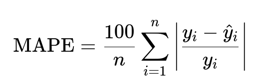
y_i is the actual sale price, and hat{y}_i is the predicted price. Lower MAPE indicates higher accuracy. MdPE provides another viewpoint on whether predictions skew too high or too low.
Comparisons should measure error differences between a baseline model that does not perform sophisticated imputation and the new model that incorporates DAE-imputed features. For homes with multiple missing attributes, extra caution is needed. Too many imputed features can degrade performance if the autoencoder cannot accurately predict them. Observing the correlation between the number of imputed fields and final MAPE or MdPE changes is a good approach.
Scalable Production Deployment
The aggregator’s engineering pipeline might use distributed scheduling frameworks. Building a containerized workflow on Kubernetes or a similar platform helps with portability. A typical approach:
Training pipeline: Batches data, creates geospatial features, trains the DAE, and stores the trained model.
Inference pipeline: Reads new or existing homes’ data, masks unknown or corrupt fields, passes them through the DAE, and outputs complete feature sets for the price-prediction model.
Decoupling training from scoring allows real-time or batch inference at scale. A stateless DAE scoring service can process one home or many homes in parallel.
Follow-up Question 1
How would you decide which features require imputation for this project?
Answer
Domain knowledge points to features highly correlated with price, including square footage, bedroom/bathroom counts, build year, lot size, and location-based data. Features with small correlations or minimal importance for predictive tasks need less attention. Focusing on strongly predictive attributes first ensures that imputation benefits the final price model. Also, the fraction of missing or noisy values in a feature is key; if many records lack that feature, a robust imputation might improve coverage and reduce bias.
Follow-up Question 2
How would you handle outliers and erroneous numerical entries before training the autoencoder?
Answer
Filtering suspicious data is crucial. Implement domain-driven thresholds for plausible property attributes. For instance, homes with more than 15 bathrooms may be flagged and replaced with a max value or removed. Log transformations or winsorizing top 1% values helps if certain features have skewed distributions. The autoencoder then encounters more stable data, reducing the chance of learning spurious patterns from extreme outliers.
Follow-up Question 3
What would you do if the autoencoder’s imputation errors degrade your final price model on certain subsets of data?
Answer
Examining subsets that degrade is the first step. Possibly those subsets (like rural properties or luxury homes) differ significantly. Creating separate specialized autoencoders for those segments or adding domain-specific features that capture their unique distributions can improve performance. Another approach is to keep the original values for subsets where the autoencoder’s predicted values do worse than a baseline imputation, such as a median or kNN approach.
Follow-up Question 4
Why consider a variational autoencoder if the denoising autoencoder is already giving good results?
Answer
A variational autoencoder (VAE) approximates data distributions in a latent space, potentially generating more diverse samples. If data has complex multi-modal distributions (e.g., certain attributes differ dramatically by region), a VAE might better capture those distributions. That said, VAEs add computational overhead. If the DAE already performs strongly, the added complexity may not be worth it unless the data’s generative aspects (such as simulating new homes or dealing with extreme missingness) are critical.
Follow-up Question 5
How would you justify the added complexity of neural network–based methods compared to simpler statistical imputation?
Answer
High-dimensional tabular data with strong non-linear and regional interactions often outperforms simpler mean/median or kNN-based approaches under neural network techniques. If simpler methods fail to capture relationships (e.g., interactions between bedroom count, square footage, and region), the NN-based approach is justified. Empirical performance improvement on MAPE and MdPE is the best proof. Careful A/B testing that shows consistent gains is the final justification.
Follow-up Question 6
How do you ensure that the imputation pipeline remains flexible for future data updates or new features?
Answer
Design the pipeline with modular steps for data pre-processing and model training. Avoid hard-coded assumptions about feature presence. Implement each step as a containerized microservice or function that reads schemas dynamically. If new columns appear, adapt the embedding layer or the input layer dimension. Maintain stateless scoring so you can deploy updated models without rewriting large parts of the pipeline. Parameterizing transformations ensures each step adjusts if data formats shift.
Follow-up Question 7
What specific metrics or thresholds would you monitor in production to confirm the continued health of this imputation approach?
Answer
Monitoring reconstruction loss over time and comparing it to historical baselines catches drift if data distributions change. Tracking real-time MAPE or MdPE on recent transactions helps confirm that overall price accuracy remains stable. Watching the fraction of homes that require heavy imputation flags potential data ingestion issues. Checking frequency distributions of imputed attributes against expected domain ranges can detect breakdowns in the model or data pipeline.