
ML Case-study Interview Question: Two-Tower Networks for Unified, Personalized Social Account Recommendations.

Browse all the ML Case-Studies here.
Case-Study question
A major social media platform wants to improve the relevance of recommended accounts to follow. They currently rely on multiple narrow candidate sources (graph-based expansions, collaborative filtering, etc.). Each source captures only a single aspect of a user’s interests. This leads to disjoint candidate recommendations that can miss the broader patterns in user preferences.
They want a unified model-based system that can incorporate multiple signals (e.g., user behavioral features, account-level features, graph-based features) into a single candidate generation pipeline. The goal is to produce a set of relevant accounts for a given user, which later gets refined by a ranking model. How would you design and implement such a model-based candidate generation pipeline from scratch, ensuring high scalability, modularity, and personalization?
Explain your approach in detail. Clarify how you will integrate various input features, handle training and inference at scale, and measure success.
Proposed Solution
Model-Based Candidate Generation
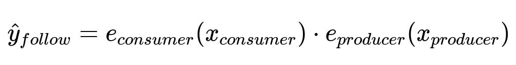
A model-based approach can learn a single embedding space where users (consumers) and recommended accounts (producers) are projected. This allows the system to unify multiple signals under one framework. A two-tower neural network is well-suited. One tower represents the user’s (consumer’s) features, and the other tower represents the account’s (producer’s) features.
Two-Tower Architecture
The consumer tower ingests user-level signals: content topics, geolocation information, language, known user interactions (e.g., follows, favorites, recents), and other engagement metrics. Each feature can be embedded into a vector space, then combined through fully connected layers. The final layer outputs a consumer embedding.
The producer tower ingests account-level signals: aggregated follower traits, embedding representations for the account, aggregated geo-based statistics, and other summary metrics. These features also go through their own embedding layers and fully connected layers. The final layer outputs a producer embedding.
Where:
e_{consumer}(x_{consumer}) is the output embedding from the consumer tower, given user features x_{consumer}.
e_{producer}(x_{producer}) is the output embedding from the producer tower, given account features x_{producer}.
The dot product reflects how likely a user is to follow a particular account.
During training, the label is whether the user actually followed that account. Minimizing a suitable loss (e.g., a logistic loss) encourages embeddings of matches (followed pairs) to be more similar.
Training
Collect user-account pairs (consumer-producer pairs) with a follow label. Include negative samples (pairs where a user did not follow a certain account) for contrast. Split data into training, validation, and test sets. Shuffle training samples to reduce bias. Train the two towers jointly by backpropagating the loss from the dot-product output.
Generate mini-batches that contain user features and account features. The training loop:
Encode user features in the consumer tower to get e_{consumer}.
Encode account features in the producer tower to get e_{producer}.
Compute dot(e_{consumer}, e_{producer}) for each pair in the batch.
Compute the loss (logistic or cross-entropy) using the observed follow label.
Backpropagate gradients to update both towers.
Inference
To generate candidates for a given user:
Compute the user’s embedding by running consumer features through the consumer tower.
Retrieve the nearest account embeddings by scanning a large bank of producer embeddings. Approximate nearest neighbor search can help, especially for millions of accounts.
The resulting top-k nearest accounts become candidates for follow suggestions.
Adding Multiple Signals
The two-tower approach enables flexible addition of new features. New user signals (e.g., new engagement metrics) can be appended to the consumer tower’s input. New account signals (e.g., fresh graph aggregates) can be appended to the producer tower’s input. The model incorporates interactions between these features by training the embedding layers and subsequent fully connected layers.
Measuring Success
Offline evaluation compares precision, recall, and ranking metrics (like mean average precision) on a validation set. Online experiments measure engagement metrics: follow rates, retention, and long-term engagement. This ensures that the model’s output is relevant.
Example Code Snippet
Below is a sketch in Python-like pseudocode:
import torch
import torch.nn as nn
import torch.optim as optim

class ConsumerTower(nn.Module):
    def __init__(self, consumer_feature_dims, hidden_dims):
        super().__init__()
        self.embeddings = nn.ModuleList([nn.Embedding(dim, embed_size)
                                         for dim, embed_size in consumer_feature_dims])
        self.fc_layers = nn.Sequential(
            nn.Linear(sum(embed_size for (_, embed_size) in consumer_feature_dims), hidden_dims[0]),
            nn.ReLU(),
            nn.Linear(hidden_dims[0], hidden_dims[1]),
            nn.ReLU(),
            nn.Linear(hidden_dims[1], 256)  # final embedding dimension
        )

    def forward(self, x):
        embedded_list = []
        for i, embedding in enumerate(self.embeddings):
            embedded_list.append(embedding(x[i]))
        combined = torch.cat(embedded_list, dim=1)
        out = self.fc_layers(combined)
        return out

class ProducerTower(nn.Module):
    def __init__(self, producer_feature_dims, hidden_dims):
        super().__init__()
        self.embeddings = nn.ModuleList([nn.Embedding(dim, embed_size)
                                         for dim, embed_size in producer_feature_dims])
        self.fc_layers = nn.Sequential(
            nn.Linear(sum(embed_size for (_, embed_size) in producer_feature_dims), hidden_dims[0]),
            nn.ReLU(),
            nn.Linear(hidden_dims[0], hidden_dims[1]),
            nn.ReLU(),
            nn.Linear(hidden_dims[1], 256)  # final embedding dimension
        )

    def forward(self, x):
        embedded_list = []
        for i, embedding in enumerate(self.embeddings):
            embedded_list.append(embedding(x[i]))
        combined = torch.cat(embedded_list, dim=1)
        out = self.fc_layers(combined)
        return out

class TwoTowerModel(nn.Module):
    def __init__(self, consumer_tower, producer_tower):
        super().__init__()
        self.consumer_tower = consumer_tower
        self.producer_tower = producer_tower

    def forward(self, consumer_x, producer_x):
        consumer_embed = self.consumer_tower(consumer_x)
        producer_embed = self.producer_tower(producer_x)
        dot_product = torch.sum(consumer_embed * producer_embed, dim=1)  # dot product
        return dot_product

# Example of usage:

consumer_tower = ConsumerTower(consumer_feature_dims=[(50000, 64), (200, 32)], hidden_dims=[512, 256])
producer_tower = ProducerTower(producer_feature_dims=[(50000, 64), (100, 16)], hidden_dims=[512, 256])
model = TwoTowerModel(consumer_tower, producer_tower)

optimizer = optim.Adam(model.parameters(), lr=1e-3)
loss_function = nn.BCEWithLogitsLoss()

# Training step
for consumer_batch, producer_batch, label_batch in data_loader:
    optimizer.zero_grad()
    logits = model(consumer_batch, producer_batch)
    loss = loss_function(logits, label_batch)
    loss.backward()
    optimizer.step()
1) How would you scale nearest neighbor retrieval for millions of accounts?
Approximate nearest neighbor indexing is crucial. Precompute producer embeddings offline or periodically. Store them in a library like FAISS or Annoy. During query time, encode the user’s embedding once. Use that embedding to probe the nearest neighbor index. This significantly lowers search time complexity compared to brute force. Sharding the data can help in distributed settings.
Precomputation steps:
Periodically batch-process all producer embeddings.
Store them in a vector index (e.g., FAISS with an IVF index or HNSW).
Choose an embedding dimension that balances representation power with computational overhead.
At inference time:
Encode the user’s features once.
Search for the top-k neighbors in the index. The output is a set of candidate account IDs.
Sharding considerations:
Split the producer embedding store by region or topic to localize search.
Maintain balanced shards. Route user embedding queries to the relevant shard or sub-index.
Caching:
For users with similar features, caching can reduce repeated searches for nearly identical embeddings.
2) How do you handle cold-start users with insufficient historical data?
Augment new user features with broader signals:
Language or location: Use location-based or language-based feature embeddings for cold-start.
Topic or interests: Let the user pick a few interest categories at onboarding. Those interest embeddings feed the consumer tower.
Default embedding: Initialize embeddings for brand-new users using aggregated stats of typical new-user behaviors.
Transfer learning:
Train on all user data but maintain a special embedding for new-user tokens, capturing average behavior patterns.
Fine-tune as soon as real engagement signals appear.
Ensure that the system updates the user embedding frequently in the early stages. Early user interactions can shape the embedding quickly.
3) How do you monitor and evaluate performance in an online setting?
Use A/B testing with real traffic. Randomly split users into control (old approach) and treatment (new model). Track:
Click-through rates on recommended accounts.
Follow conversions.
Engagement metrics: how many recommended accounts are actually followed, retweeted, or interacted with.
Long-term retention: do users keep following recommended accounts over time?
Compare these metrics between control and treatment. If the new model statistically outperforms the old pipeline, roll it out. Monitor user feedback for unexpected biases or quality issues.
4) How do you optimize the framework for adding new features quickly?
Design the input pipeline to modularly ingest new features. Build each tower with:
Dedicated embedding layers for each new feature.
Automatic shape/dimension checks for easy plugging-in of new embeddings.
Well-documented data sources for each feature.
Version the training data schema. Adopt feature stores to ensure consistent transformations between training and inference. Continuous integration pipelines can automatically retrain the model whenever new features are introduced.
5) Why not rely on separate specialized candidate sources?
Multiple specialized sources create a fragmented system:
Harder maintenance overhead: each source requires unique logic.
Limited capacity to combine signals: combining sources in downstream steps can miss deeper interactions.
A two-tower approach merges signals into a single embedding space, capturing cross-feature relationships end-to-end.
This unified approach increases personalization and can simplify the entire candidate generation flow.
6) How do you address potential issues of popularity bias or diversity in the recommended accounts?
Popularity bias can occur when large accounts dominate. Encourage diversity:
Penalize extremely popular accounts in the loss function or re-rank final recommendations with a diversity regularizer.
Calibrate recommendations so new or niche accounts are not overshadowed.
Post-processing re-ranking could incorporate a popularity-based discount factor or a novelty score.
Measure final diversity metrics (e.g., coverage of different topics or smaller accounts) in A/B tests to ensure a balanced set of suggestions.
7) Could you handle real-time user updates?
Embed dynamic user signals: recency of interactions or changing interests. Update the consumer embedding in near-real time using streaming data. Periodically refresh the producer embeddings. Use incremental or mini-batch updates for those accounts. If full real-time updates are expensive, blend approximate real-time signals (like streaming counters) with the last stored embeddings.
If the system must react within minutes to user actions, set up streaming pipelines that recompute embeddings for consumer or producer towers. Or do partial updates: only re-encode the user’s tower while producer embeddings update on a slower schedule.
8) What if the dot product saturates and does not sufficiently capture complex interactions?
Try deeper interactions:
Additional MLP layers after the concatenation of e_{consumer} and e_{producer}.
Factorization machines or deep factorization approaches to capture feature cross terms.
Alternate similarity metrics, e.g., gating layers or attention-based approaches.
Experiment with different pooling strategies (like element-wise multiplication or co-attention) if dot product alone underperforms. Conduct offline experiments to see which architecture best generalizes.
9) How do you ensure fairness and mitigate algorithmic bias?
Collect representative data from diverse user segments. Include fairness-focused metrics (e.g., group-level acceptance rates) in your evaluation. Check if the model systematically favors specific groups. Potentially incorporate fairness-aware training objectives or constraints. Periodic audits ensure that the recommendations remain balanced across demographic or interest groups.
10) How do you handle training data imbalance for highly popular accounts?
Include a sufficient variety of negative samples. Oversample underrepresented examples. Use more sophisticated sampling strategies:
Weighted negative sampling to emphasize rare or niche accounts.
Balanced mini-batch composition so that the model doesn’t overfit to majority classes.
Monitor the distribution of follow vs. non-follow pairs. Perform thorough offline checks for recall on less popular accounts.