ML Interview Q Series: Accelerating and Stabilizing Deep Network Training with Batch Normalization.

📚 Browse the full ML Interview series here.

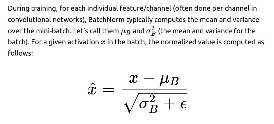
3. Batch Normalization: What is Batch Normalization and how does it help in training deep neural networks? Explain how batch norm normalizes the inputs of each layer (mean 0, variance 1 during training) and discuss its effects on training speed and stability. Also, clarify how BatchNorm’s behavior differs between training and inference.

Understanding Batch Normalization in Deep Neural Networks

Batch Normalization (BatchNorm) is a technique introduced to address problems such as internal covariate shift and training instability in deep neural networks. It normalizes the intermediate outputs of layers, thereby stabilizing and accelerating training. This normalization also allows for higher learning rates, mitigates vanishing or exploding gradients, and generally improves network generalization.

How Batch Normalization Works

The main idea is to normalize activations for each training mini-batch such that the outputs of a layer have zero mean and unit variance, and then to allow the network to learn any necessary shift or scale of those normalized outputs.

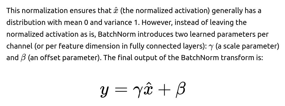
These learnable parameters γ and β allow the network to recover any useful shift or scale that might be beneficial for representing the data effectively. In other words, while normalization helps with stable gradients, the network can still shape these normalized values in a flexible manner.

Why It Helps with Training Speed and Stability

BatchNorm reduces the problem commonly referred to as “internal covariate shift,” where the distribution of intermediate activations in a deep network changes during training as the parameters in the previous layers update. By enforcing a consistent distribution of activations within a batch, the parameters in subsequent layers see more stable inputs. This stability means:

Faster Convergence. Because the intermediate outputs seen by deeper layers are more consistent across different updates, gradient descent can converge faster. Networks often train successfully even with relatively high learning rates.

Improved Gradient Flow. Normalizing helps control the scale of the outputs going into subsequent layers, thus making the gradients more stable as they backpropagate. This stabilization can mitigate exploding or vanishing gradients.

Better Generalization. Empirical evidence suggests that BatchNorm can help models generalize, possibly because it adds a form of noise (through small batch variations) and regularization, although the exact mechanism is still an area of ongoing discussion.

Differences Between Training and Inference

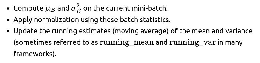
During training, BatchNorm uses the mini-batch’s mean and variance to normalize activations. However, at inference time (when the model is deployed and sees just a single sample or a different batch size distribution), we don’t compute statistics from a single test sample or a smaller batch. Instead, we use “running estimates” or “moving averages” of the mean and variance collected over the training process. Concretely:

In training mode:

In inference mode:

• The running (moving) average of the mean and variance are used to normalize the test data instead of the current batch’s statistics. That way, each test sample sees a consistent transformation based on the entire training data’s estimated statistics.

• The parameters γ and β remain the same learned scale and shift from training.

If we did not have these running estimates, inference could be unstable when the batch size is small or the data distribution at test time is very different. Using the averaged global statistics ensures consistent and well-defined normalization.

Potential Implementation in Python (using PyTorch-like pseudocode)

import torch
import torch.nn as nn

class CustomBatchNorm(nn.Module):
    def __init__(self, num_features, epsilon=1e-5, momentum=0.1):
        super(CustomBatchNorm, self).__init__()
        self.num_features = num_features
        self.epsilon = epsilon
        self.momentum = momentum

        # Learnable scale and shift parameters
        self.gamma = nn.Parameter(torch.ones(num_features))
        self.beta = nn.Parameter(torch.zeros(num_features))

        # Running estimates used for inference
        self.running_mean = torch.zeros(num_features)
        self.running_var = torch.ones(num_features)

    def forward(self, x):
        if self.training:
            # Compute mean and var across batch and spatial dimensions
            batch_mean = x.mean(dim=(0,2,3), keepdim=True)  # for conv2d case
            batch_var = x.var(dim=(0,2,3), unbiased=False, keepdim=True)

            # Update running estimates
            self.running_mean = (1 - self.momentum) * self.running_mean + self.momentum * batch_mean.squeeze()
            self.running_var = (1 - self.momentum) * self.running_var + self.momentum * batch_var.squeeze()

            # Normalize
            x_hat = (x - batch_mean) / torch.sqrt(batch_var + self.epsilon)
        else:
            # Use running estimates during inference
            x_hat = (x - self.running_mean.view(1, -1, 1, 1)) / \
                    torch.sqrt(self.running_var.view(1, -1, 1, 1) + self.epsilon)

        # Scale and shift
        out = self.gamma.view(1, -1, 1, 1) * x_hat + self.beta.view(1, -1, 1, 1)
        return out

Here, in training mode, we compute batch_mean and batch_var for each feature across the batch and spatial dimensions. Then we apply the normalization step. We also update running_mean and running_var. In inference mode (model.eval()), we do not compute the batch statistics but use running_mean and running_var to normalize the input.

How This Addresses Common Pitfalls

Helps networks train faster. Normalizing each layer’s input means less “oscillation” in activation distributions, so the training can stabilize quickly. This often cuts down the number of epochs needed for convergence.

Reduces exploding/vanishing gradients. By controlling the scale of each mini-batch’s activations, gradient backpropagation is more stable, leading to a healthier optimization process.

Allows higher learning rates. Because the inputs to deeper layers remain in a stable distribution, higher learning rates can be used without blowing up the training.

Potential Issues and Considerations

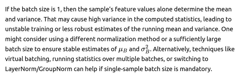
Small batch sizes. If the batch size is too small, estimates of mean and variance may be noisy, which can degrade performance or cause instability. Specialized techniques like Group Normalization or Layer Normalization can help in such cases.

Sequence data and RNNs. For recurrent architectures dealing with sequential data, classic BatchNorm might not be an optimal solution because temporal dependencies can complicate how batches are formed. LayerNorm or other normalization techniques are often used for RNNs.

Distribution shift. If there is a huge shift in data distribution between training and inference, the running mean and variance may no longer be representative of the real test distribution. Careful domain adaptation or fine-tuning might be required.

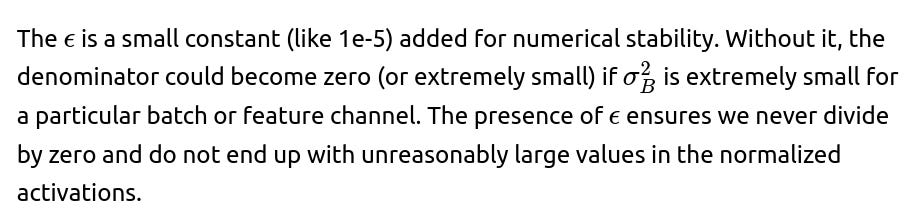
Precision. The computation of the variance can cause numerical instabilities when the variance is very small or the data is large in magnitude. The addition of ϵ helps mitigate division-by-zero or extremely large division values.

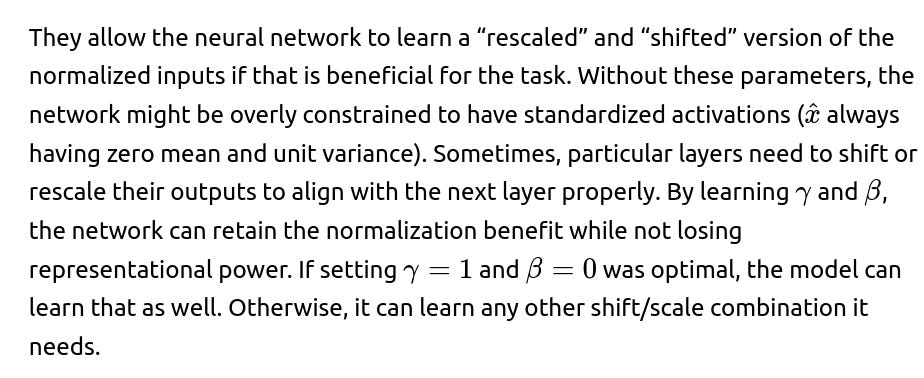
Common Follow-up Question: Why Are γ and β Needed?

Common Follow-up Question: How Does BatchNorm Differ from LayerNorm or InstanceNorm?

While BatchNorm normalizes across the batch dimension (and spatial dimension in convolutional layers) for each feature, LayerNorm normalizes across the features for each individual sample, and InstanceNorm normalizes each sample channel by channel. This difference matters especially when the batch size is small or when dealing with sequence data. LayerNorm is often preferred for RNNs because it normalizes across the feature dimension for a single time step, which works better for recurrent connections. InstanceNorm is common in style transfer tasks where each individual sample’s normalization is more relevant. GroupNorm is somewhere in between, grouping certain channels together for normalization.

Common Follow-up Question: What Happens if the Batch Size is 1 During Training?

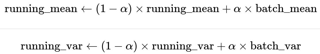
Common Follow-up Question: How Do We Update the Running Mean and Variance?

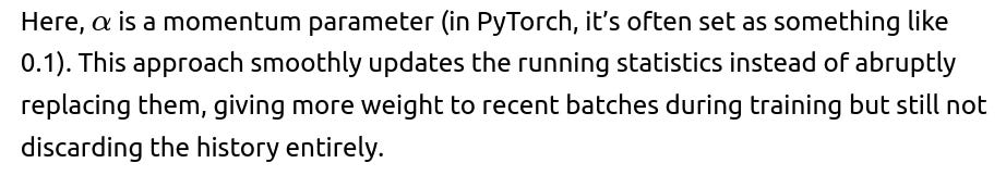
In frameworks like PyTorch or TensorFlow, the update is often performed using exponential moving averages:

Common Follow-up Question: Is It True That BatchNorm Also Regularizes the Model?

In practice, yes, though it was not the original motivation. BatchNorm introduces some noise in the normalization process because each mini-batch can slightly differ in its statistical properties. This acts similarly to a regularizing effect (akin to dropout’s noise) and can improve generalization. However, whether or not it is a “pure regularizer” depends on the scenario, and it may not always be sufficient as a standalone regularization technique.

Common Follow-up Question: How Does BatchNorm Behave in Residual Networks?

Residual networks often place BatchNorm right after each convolution and before the ReLU nonlinearity. The arrangement typically goes: Convolution -> BatchNorm -> ReLU. This helps keep signals flowing stably through the skip connections, ensuring that gradients propagate cleanly. Empirical work has shown that using BatchNorm in residual blocks is crucial to stabilizing very deep networks like ResNet-50/101/152.

Common Follow-up Question: What Happens If the Data Distribution Changes Significantly After Deployment?

If a large domain shift occurs, the running mean and variance (which were computed during training) might become inaccurate. This can degrade model performance because the normalizing transformation no longer matches the new data distribution. Approaches to handle this include:

• Fine-tuning: Recompute or partially update the running statistics on new data (if labels or partial labels are available).

• Domain adaptation methods: Adjust model parameters or BatchNorm statistics to align with the new domain.

Common Follow-up Question: Can BatchNorm Improve Gradient-Based Optimization in Very Deep Networks?

Yes. In extremely deep networks, the chain of gradients can degrade quickly. By normalizing each layer’s inputs, BatchNorm ensures that the scale of the gradients is relatively controlled across layers, reducing issues like exploding or vanishing gradients. This stability is particularly beneficial as the network depth grows large.

Common Follow-up Question: What Is the Effect of BatchNorm When Used with Dropout?

BatchNorm and Dropout can be combined, but their order matters. Many practitioners place BatchNorm before Dropout. This is because Dropout randomly zeroes out activations, which can influence the mean/variance if done before the normalization step. Others experiment with different placements. Empirically, placing Dropout after BatchNorm is common, but the best arrangement can be task-dependent. Modern networks sometimes rely less on Dropout and more on BatchNorm because BatchNorm itself has a mild regularizing effect.

Common Follow-up Question: Could We Have Merely Standardized the Input Data Instead of Using BatchNorm?

Preprocessing your dataset features to have zero mean and unit variance is a good idea, but that does not solve the issue that intermediate features in deeper layers can shift as training progresses. BatchNorm addresses the shifting distributions that occur within the network layers themselves during optimization. The dynamic, per-batch normalization is key to controlling these shifts, which simple data-level standardization cannot address once data flows deeper into the network.

Common Follow-up Question: Are There Cases Where We Should Avoid BatchNorm?

If batch sizes are extremely small or if the data is sequential with strong temporal dependencies (like in certain RNN applications), BatchNorm may not be ideal. The estimates of mean and variance for each batch will be unreliable or may degrade performance. Alternative normalizations such as LayerNorm, InstanceNorm, GroupNorm, or carefully tuned techniques might be preferable.

Common Follow-up Question: Why Is There an ϵϵ in the Denominator?

Common Follow-up Question: How Does Momentum in BatchNorm Differ from the Usual Momentum in Optimizers?

Momentum in BatchNorm (often a parameter named momentum in frameworks) controls how quickly the running estimates of mean and variance are updated. This is separate from the momentum used by stochastic gradient descent or other optimizers. A larger BatchNorm momentum parameter means the running estimates reflect the current batch statistics more strongly (giving them more weight). A smaller momentum means the running estimates change more slowly over time.

Common Follow-up Question: Does BatchNorm Solve All Issues of Deep Neural Network Training?

While BatchNorm is extremely beneficial, it doesn’t solve every problem. You still might encounter vanishing gradients if you have extremely deep networks with certain architectural choices, or you may still need carefully tuned learning rates and weight initializations. In some cases, alternative normalizations might be superior. However, in practice, BatchNorm is one of the most widely used techniques because it offers significant benefits with relatively minor downsides in typical convolutional and feed-forward architectures.

Common Follow-up Question: Why is the Beta Parameter Needed if We Already Have a Bias Term in the Next Layer?

While it might seem redundant, the shift (β) in BatchNorm is independent of the linear transformation’s bias in the next layer. The bias in the next layer is added before or after a convolution/fully-connected operation, whereas the shift in BatchNorm is applied after the normalization step. Additionally, conceptually, β helps ensure that BatchNorm can represent any shift needed to align the normalized distribution with beneficial activation regions (e.g., placing normalized values where ReLU or other nonlinearities operate effectively), which might not always be the same shift learned by the next layer’s bias. Although in principle one could sometimes combine these shifts, in practice the separate β in BatchNorm consistently improves training stability.

Common Follow-up Question: How Does BatchNorm Compare to Weight Initialization Techniques?

Weight initialization helps ensure that early activations and gradients are neither too large nor too small. BatchNorm further stabilizes the distribution of activations as the network continues training, whereas weight initialization is a one-time fix at network startup. They are complementary: good weight initialization plus BatchNorm typically lead to faster and more robust convergence.

Common Follow-up Question: Are There Any Theoretical Guarantees or Proofs That BatchNorm Always Helps?

The exact theoretical reasons for BatchNorm’s effectiveness are still a subject of active research. There are partial explanations: it reduces internal covariate shift, it smooths the loss landscape, etc. Empirically, it almost always helps in convolutional neural networks and many MLP-based architectures, making it a near-standard technique. However, there can still be corner cases or tasks where BatchNorm yields minimal gains or is outperformed by alternatives.

Common Follow-up Question: Can We Fix γ and β Instead of Making Them Learnable?

Sometimes, for certain tasks, one might fix γ=1 and β=0, effectively removing the learnable parameters and just normalizing. This can simplify the model, but it might limit representational capacity. In many real-world applications, letting γ and β be learned is best practice. They can effectively adapt the normalized distribution to the best range for the subsequent layers.

Common Follow-up Question: How Would You Debug a Model That Has a Suspected BatchNorm Problem?

One approach is to:

• Check the running means and variances to see if they have “blown up” or are not being updated as expected.

• Try disabling BatchNorm’s updates (fix the statistics) to see if that stabilizes or destabilizes training, diagnosing if the updates themselves are causing issues.

• Confirm that the batch size is large enough for reliable statistics.

• If small batch size is unavoidable, test GroupNorm or LayerNorm to see if training stabilizes.

• Check if the architecture or data pipeline is inadvertently mixing training and evaluation modes (e.g., always keep model.train() vs. model.eval() states correct).

• Inspect if the momentum parameter is set to a strange value that could hamper stable updates.

Common Follow-up Question: Does the Order of Operations (Conv -> BN -> ReLU) Matter?

Yes, usually BN is placed after convolution (or fully-connected layer) but before the nonlinear activation (ReLU, etc.). This is the standard pattern: it normalizes the outputs from the layer’s linear operation, then the activation function is applied. If BN is placed after ReLU, the distribution might be skewed by the nonlinearity, and the effect of normalization might not be as directly beneficial.

Common Follow-up Question: Could We Just Use a Single Global Mean and Variance for the Entire Dataset?

That would be akin to a global data normalization, but it wouldn’t dynamically adapt to each mini-batch during training. Doing so could hamper the benefits we derive from controlling the distribution shift within each batch. Also, different batches might have different distributions, especially in non-i.i.d. settings. One advantage of BatchNorm is that it handles these local variations while still preserving global running estimates for inference.

Common Follow-up Question: How Does BatchNorm Interact with Skip Connections in Residual Blocks?

BatchNorm typically appears after each convolution (and sometimes right before adding the skip-connection output). This ensures that both the main path and skip path remain well-scaled. Empirical results from the original ResNet paper and subsequent research show that having BatchNorm in each of these segments is critical for stable training, especially as depth increases.

Common Follow-up Question: Is It Necessary to Drop the Bias Term in Convolution Layers When Using BatchNorm?

In many frameworks, if you apply BatchNorm immediately after a convolution, the convolutional layer’s bias parameter is often redundant because BatchNorm’s shift (β) can accomplish a similar effect. Practitioners sometimes remove biases from convolution layers to slightly reduce parameter count and training time. It typically does not harm performance. That said, in standard frameworks, you might leave the bias on by default, and it usually does not significantly impact performance either way.

Common Follow-up Question: Are There Any Memory or Computation Drawbacks?

BatchNorm requires additional memory to store the moving mean and variance, plus small overhead for computing per-batch statistics. Typically, this overhead is negligible compared to the overall memory usage of the model and the forward/backward passes. The benefits of stable training usually far outweigh any small overhead.

Common Follow-up Question: What If the Model Overfits After Adding BatchNorm?

While BatchNorm can have a mild regularizing effect, it does not guarantee prevention of overfitting by itself. If overfitting arises, consider standard strategies: more data, stronger regularization, dropout, data augmentation, or reducing model complexity. BatchNorm alone may not be sufficient to cure overfitting in all cases.

Common Follow-up Question: Could We Use BatchNorm for Non-Neural Network Models?

BatchNorm is designed for networks that learn transformations of intermediate activations. It’s most useful for deep neural networks, especially convolutional ones. For simpler models (e.g., logistic regression, random forests, classical SVMs), the notion of normalizing each mini-batch at intermediate layers is not typically relevant because those models don’t have internal layers that transform data in the same sense as a deep network.

Common Follow-up Question: Do We Need to Recalculate BatchNorm Statistics After Fine-tuning on Another Dataset?

Yes, it’s often recommended to either:

• Fine-tune the entire model, letting the BatchNorm statistics update on the new dataset.

• Freeze the previously learned BatchNorm statistics if the new dataset is small and we don’t want them to overfit to the smaller domain.

The choice depends on how different the new dataset is and whether you have enough new data to get stable estimates of mean/variance.

Common Follow-up Question: What If We Use BatchNorm Layers in Generative Models?

For generative adversarial networks (GANs), BatchNorm is frequently employed to stabilize training for both the generator and discriminator. However, certain variants of GAN architectures avoid it in the discriminator to reduce correlations across samples in a mini-batch. Some specialized norms like LayerNorm or PixelNorm might be used instead, depending on the architecture. Overall, BatchNorm can still help generative models converge, but the exact effect depends on how the training dynamics are set up.

Common Follow-up Question: Could BatchNorm Hurt Performance if We Don’t Handle It Properly?

Yes. Incorrect usage, especially forgetting to switch between training (model.train()) and inference (model.eval()), leads to using the wrong statistics for normalization during inference. Or if the batch size is extremely small, the statistics might be too noisy. A mismatch in training/inference mode or an incorrectly set momentum parameter can degrade performance.

---

Below are additional follow-up questions

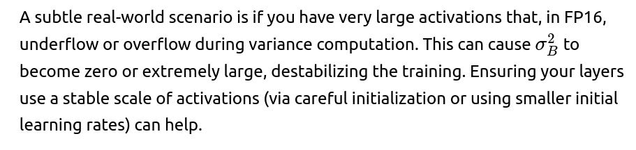
What Are Some Potential Issues When Using BatchNorm in Half-Precision (FP16) Training?

When training in half-precision, numerical stability becomes more critical. In half-precision (FP16), the dynamic range is reduced, and floating-point operations can lose accuracy faster than in single precision (FP32). In BatchNorm, the division by the batch variance (which could be a small number) plus an ϵ term can cause rounding errors that are magnified in half-precision. This can lead to unstable or inaccurate gradients.

One common strategy to mitigate these issues is “mixed-precision” training, where certain operations (like convolution and matrix multiplication) are done in FP16 for speed and memory gains, but BatchNorm’s statistics and possibly the final “master” weights are stored in FP32. The reason is that the computation of mean and variance can be more stable in FP32. Frameworks like PyTorch have built-in automatic mixed-precision utilities that handle some of these details behind the scenes, keeping BatchNorm in a more stable precision while still allowing the rest of the network to benefit from the performance advantages of FP16.

How Does BatchNorm Behave in a Distributed Training Environment with Multiple GPUs or Multiple Machines?

In distributed training, each GPU (or machine) may process a different mini-batch of data, meaning each replica computes separate batch statistics (mean and variance). Typically, the default approach is to compute BatchNorm statistics (mean and variance) separately on each replica, which can result in slightly different updates. This is called “replica BatchNorm.”

If the batch size per replica is very small, the statistics might be noisy. Some frameworks offer “synchronized BatchNorm” or “global BatchNorm,” where all replicas’ statistics are aggregated so that the mean and variance are computed over the global batch across GPUs. This gives more stable statistics when each GPU sees only a small fraction of the total mini-batch.

The trade-off is that synchronized BatchNorm can introduce communication overhead, potentially reducing the training speed. It may still be worth it if your overall batch size per device is very small, because the more stable gradient updates can outweigh the communication cost. In large-scale training, with large batches per device, standard “replica BN” might suffice because each replica’s batch dimension is large enough for stable statistics.

A subtle pitfall is forgetting to toggle the same training/evaluation mode across all distributed processes. If some processes are in training mode and others in eval mode, the running means and variances can get out of sync across replicas.

If We Freeze the BatchNorm Parameters Mid-Training, What Effects Might We Observe?

Sometimes, practitioners freeze the BatchNorm parameters (meaning they stop updating the running mean, running variance, and the learnable γ and β) after a certain stage of training. This can happen in transfer learning, where the original dataset’s batch statistics are considered “good enough” for the new task, and further updates might degrade them if the new dataset is small.

If you freeze the running mean and variance, the network will always use the same statistics for normalization, which can provide a consistent data distribution to deeper layers. This might improve stability if your new training data is limited. However, if the new data distribution differs significantly from the old one, using the old statistics can hurt performance. Freezing γ and β may also limit the model’s flexibility in adjusting to new data. The subtlety is balancing the risk of overfitting the new domain’s batch statistics (especially with small data) versus ignoring distribution differences by freezing.

In practice, a partial freeze is sometimes done: keep γ and β learnable but freeze the running statistics, or vice versa. The effect depends strongly on how different the new domain is and how big your new training set is.

What Is the Effect of BatchNorm on Interpretability and Visualization of Feature Maps?

BatchNorm standardizes activations, which can make direct comparisons of raw feature-map intensities less interpretable across layers or across different training steps because the statistics are shifting to maintain mean 0 and variance 1 within each batch. Suppose you want to visualize and compare the activation magnitudes from layer to layer or over time; BatchNorm’s dynamic rescaling can obscure direct comparisons of absolute values.

On the other hand, BatchNorm might allow you to interpret normalized features more consistently within a given layer, because you know that within each batch, features are zero-mean and unit-variance before γ and β. Some practitioners argue this can simplify certain forms of analysis or interpretability, because the distribution of raw normalized features is somewhat standardized. However, the presence of learnable γ and β reintroduces a shift and scale, potentially complicating direct raw-value interpretation.

A subtle real-world example is if you rely on absolute activation levels for certain saliency or attribution methods. The transformations from BatchNorm might require additional steps (like applying the inverse transformation) to get the original unnormalized feature magnitudes.

How Does BatchNorm Interact with Gradient Accumulation or Micro-Batching?

When using gradient accumulation or micro-batching, you might process a batch in smaller chunks (micro-batches) for memory reasons, then accumulate gradients over several forward-backward passes before updating parameters. If BatchNorm is present, the mean and variance are typically computed at each micro-batch step, not over the entire effective batch. This can introduce a discrepancy between the effective large batch size for gradient accumulation and the small micro-batch size used to compute BN statistics.

If the micro-batch is too small, the BN statistics could be noisy, leading to unstable training. In some frameworks, there are ways to accumulate BN statistics over multiple micro-batches to approximate what would happen with a single large batch. However, this can be more complicated to implement. A potential pitfall is ignoring the effect of BN on micro-batching and wondering why training stability worsens when switching from a single large batch to multiple micro-batches.

Does BatchNorm Work Well with All Activation Functions, Such as Swish or GELU?

BatchNorm is generally agnostic to the specific choice of activation function, as it normalizes the preactivation outputs (or immediate post-convolution outputs) before applying nonlinearity. For example, with ReLU, we typically place BN before ReLU. For Swish or GELU, the standard practice of “Conv -> BN -> Activation” often still works.

A subtlety arises if the activation drastically changes the distribution shape or if the partial derivatives for that activation interact in unpredictable ways with the normalized distribution. In practice, BN has proven robust across many commonly used activation functions, though carefully monitoring training curves is important to detect any unusual behaviors. Rarely, certain custom activations might demand specialized normalization that is tailored to their nonlinearity.

Can BatchNorm Help with Catastrophic Forgetting in Continual Learning?

Catastrophic forgetting happens when a model, trained sequentially on different tasks, forgets previously learned tasks upon learning a new one. BatchNorm can indirectly influence forgetting dynamics, because the normalized activations might stabilize training across tasks. However, it does not by itself solve catastrophic forgetting. The running mean and variance might become heavily biased towards the latest task’s distribution, potentially harming performance on earlier tasks.

Some continual-learning techniques freeze or partially update BN statistics for previously learned tasks, or maintain separate BN parameters for different tasks. This approach, while more complex, can preserve the relevant normalization for each task. A pitfall is that this increases complexity and can be memory-intensive if many tasks require separate BN parameters.

How Does BatchNorm Behave in Networks That Use Attention Mechanisms?

In attention-based architectures (e.g., Transformers), it is more common to see LayerNorm than BatchNorm, because LayerNorm is invariant to sequence length and batch size. However, one can still use BatchNorm in certain hybrid architectures that combine convolutional blocks with attention. In these scenarios, BN is typically applied after convolutional layers or feed-forward sub-blocks within the network.

A subtlety is that attention modules often rely on the distribution of query/key/value features across a sequence. If you use BN inside these computations, you might inadvertently mix statistics across sequence elements in a way that disrupts the attention operation. That’s one reason LayerNorm or RMSNorm is standard in Transformers. However, for purely convolutional attention blocks, BN might still be beneficial. Thorough experimentation is required to see whether BN truly improves training stability in a given attention-based design.

How Can BatchNorm Influence Adversarial Robustness?

Adversarial robustness is the model’s resilience to small, carefully crafted perturbations in the input. Research suggests that BatchNorm can either help or hurt adversarial robustness depending on various factors, such as how it interacts with gradient flow, how the running statistics behave, and whether the adversarial examples shift the data distribution away from the learned running mean and variance.

A subtle scenario is if an attacker crafts adversarial examples that exploit the mismatch between training batch statistics and actual input distribution at test time. If the adversarial input triggers normalization behaviors different from what was seen in training, the network might misclassify. Defensive strategies could involve using robust normalization layers that clamp or limit the influence of outliers, or performing adversarial training that includes BN’s effect in the gradient pipeline. In practice, BN is not a silver bullet for adversarial robustness; specialized adversarial training methods are usually needed.

How Is BatchNorm Affected by Regularization Methods Like Weight Decay or Penalties?

The BatchNorm parameters γ and β are typically subject to the same weight decay or penalties as other parameters, unless explicitly excluded in the optimizer. If you do apply weight decay to γ and β, it can bias them towards zero over time (particularly for β). This might reduce the network’s ability to shift or scale features, potentially harming performance if the model needs a non-trivial scale or shift.

Many practitioners exclude BatchNorm parameters from weight decay, allowing them to be learned freely. Some frameworks do this by default. The subtlety is that if you have extreme overfitting concerns, you might want some regularization on γ and β, but be aware that it can degrade the benefits of having flexible scaling and shifting.

Can We Use BatchNorm Effectively in Models With Residual Connections That Skip Over Several Layers?

BatchNorm can be effective in residual networks of arbitrary skip length, as long as you consistently apply BN to the main branches where transformations occur. However, if a skip connection bypasses multiple layers that include BN, you could see a discrepancy in magnitude or distribution between the skip path and the main path. Typically, residual blocks have the pattern “Conv -> BN -> ReLU -> Conv -> BN -> add skip.” If you create deeper or more complex skip structures, ensure that BN is applied in a consistent manner.

A potential pitfall is that if the skip path is purely identity (no BN) but the main path has BN, the distributions might mismatch. Usually, the standard approach used in architectures like ResNet is stable, but custom modifications should keep an eye on distribution alignment.

What Happens If We Initialize γ and β to Non-Standard Values, Like γ=0 or β=1?

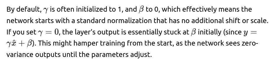
On the other hand, some initialization schemes set γ to values that reflect the expected scale of the next layer’s inputs. But typically, γ=1 is a neutral starting point. Setting β to 1 or any large value can shift the outputs significantly, requiring the earlier training steps to adapt the other parameters to compensate. This might slow early training or cause instabilities.

A real-world edge case is if your layer following BN needs a certain initial distribution. Then you might carefully initialize γ and β to match that distribution. But for most standard architectures, the default initialization is robust.

How Might BatchNorm Behave in Multimodal Architectures (e.g., Combining Images, Text, and Audio)?

In multimodal networks, each modality can have very different data distributions, especially if the inputs are processed by separate branches (e.g., an image encoder and a text encoder). Usually, each branch has its own set of BatchNorm layers with parameters learned specifically for that modality. If you try to share BN layers across modalities (which is uncommon), the distribution mismatch might degrade performance because the mean and variance for images may differ drastically from text embeddings or audio features.

A subtlety arises if you combine feature maps from multiple modalities mid-network. Then you might have to decide whether to apply BN separately per modality or after the features are fused. The latter might obscure the distinctive distribution of each modality. In practice, BN is typically done within each modality’s feature extraction path, then fusion happens at a later stage without BN.

Are There Instances Where BatchNorm Can Cause Gradient Explosions?

While BatchNorm usually reduces the risk of gradient explosions, it can exacerbate them in rare edge cases. For example, if the computed variance is extremely small (due to some unusual distribution of activations) and ϵ is too tiny, dividing by this small value can produce large normalized values, which can lead to large gradients. This typically happens if your input data or parameter initialization is pathological, or if your architecture inadvertently funnels certain inputs to produce near-constant activation in a channel. In practice, using a slightly larger ϵ can help prevent these issues.

Another subtle cause might be if γ is learned to be extremely large to maximize certain feature channels. This large γ, multiplied by a small variance normalization, can produce large outputs. Keeping an eye on the learned γ values can help detect potential gradient instability.

Does BatchNorm Influence the Optimal Choice of Optimizer Hyperparameters Like Learning Rate or Momentum?

Yes. Because BatchNorm stabilizes and rescales activations, you can often use higher learning rates without the risk of blowing up gradients. However, it doesn’t remove all sensitivity to learning rate. In many empirical studies, a combination of BatchNorm plus a well-chosen learning rate leads to faster convergence.

The momentum in your optimizer (e.g., in SGD with momentum) interacts with the BN momentum parameter for running mean/variance in a conceptually different way, so you typically tune them independently. A subtle scenario is if you set the BN momentum parameter too high (meaning you rely heavily on the current batch’s statistics) while also using a large optimizer momentum. This can lead to a mismatch where the weight updates are quite smoothed, but the BN updates jump quickly. This mismatch can cause slower overall convergence or slightly erratic BN statistic updates. Careful tuning might be required.

How Could BatchNorm Parameters Interact with a Layer That Uses WeightNorm?

WeightNorm is a technique that re-parameterizes the weight vectors in layers to decouple magnitude and direction, normalizing the weights themselves. BatchNorm, on the other hand, normalizes activations. Using both can lead to complicated interactions, because each is normalizing at different stages: one normalizes the parameters, the other the activations. Generally, they can coexist if carefully implemented.

A potential pitfall is if the combined effect of WeightNorm and BatchNorm causes certain layers to collapse in scale or to have conflicting normalization objectives. In practice, many modern architectures focus on either BN or alternative normalization for the activations, rather than mixing them with WeightNorm. If you do mix them, you must carefully monitor training, as debugging can be more complex.

Could an “Incorrect” Implementation of BatchNorm Ever Be Useful?

Sometimes, researchers experiment with variations that might appear “incorrect” compared to the standard BN definition. For instance, normalizing only across spatial dimensions in a convolutional layer but not across the batch dimension can approximate InstanceNorm. Or normalizing across the batch and feature dimensions but ignoring spatial dimensions might approximate LayerNorm in a convolution setting. These modifications might help in specific tasks like style transfer or artistic rendering.

A subtle real-world scenario is that your dataset might have certain structured noise or a very small batch size, making the standard BN approach degrade performance. A slightly unorthodox approach to computing means and variances (for example, ignoring certain outliers or weighting samples differently) might yield better performance. One must be cautious, though, because deviating from well-established BN practices can introduce new complexities and might not generalize.

Do Large Outliers in a Batch Greatly Affect the Computed Mean and Variance?

Yes. The mean and variance are sensitive to outliers. If your mini-batch contains extreme values (e.g., a corrupted image or mislabeled data with extreme pixel intensities), it can skew the batch’s mean and variance, leading to unusual normalization for that particular batch. This can cause training instabilities or degrade performance temporarily. Often, the random sampling across many epochs mitigates persistent issues, but if outliers appear frequently in your data, it can systematically disrupt training.

A subtle fix is to use a robust variant of BN that either clips outliers or uses robust statistics (like median absolute deviation). However, these are not standard in most libraries. Another approach is to carefully preprocess or remove severely out-of-range data. In a real-world scenario, data cleaning can go a long way toward preventing outlier-induced instability in BN.

How Does BatchNorm Affect Output Boundaries in Classification Problems with Very Few Classes or Very Many Classes?

In a classification setting, BN is typically done before the activation leading to the final logits. If there are very few classes (like binary classification), BN might not pose any special challenges since you still normalize the activations in hidden layers. If there are many classes (e.g., thousands of classes in large-scale classification), BN still normalizes the internal activations but does not directly change the dimension of your output layer. The presence of many classes typically affects the final layer’s parameter count more than the BN layers.

One subtle scenario is if your final layer is extremely large for a high-cardinality classification problem, the preceding BN might be crucial for preventing extremely large or skewed logits. On the other hand, in a small-class problem, the benefits of BN remain in stable optimization. You rarely see a direct conflict with the number of classes. The key is ensuring that your hidden layers and the data going into BN layers maintain enough variety and batch size so that meaningful statistics can be computed.

Are There Tricks to Improve BatchNorm’s Performance on Recurrent or Autoregressive Tasks Without Switching to LayerNorm?

Applying BN directly to RNN hidden states can be tricky because each timestep might come from a different distribution. Some partial workarounds involve carefully segmenting sequences into chunks and applying BN over those chunks. Another idea is to separate the forward pass across timesteps but keep the same BN parameters (and possibly the same mean/variance across timesteps). Still, these approaches can degrade sequence modeling capabilities because they break the temporal dependency or make training more complicated.

A subtle real-world scenario is if you have a short sequence length or a fairly large batch size dimension for your RNN. You might be able to treat each timestep as part of the batch dimension for computing BN statistics. This helps, but it can blur the boundaries of sequences. Alternatively, you can experiment with “virtual batches” or small sequence groupings. However, these approaches are less standard, and often practitioners prefer LayerNorm, which is simpler for sequence-based tasks.

Could Unsupervised Pretraining with BatchNorm Statistics Mismatch the Supervised Fine-Tuning Stage?

In unsupervised or self-supervised pretraining (e.g., autoencoder or contrastive learning tasks), your BN layers learn statistics from unlabeled data. When you fine-tune the model on labeled data, the distribution might shift if the labeled subset differs from the unlabeled portion or if the task changes drastically. This can lead to a mismatch between the BN’s running statistics and the new data distribution.

A subtle fix is to either update BN statistics again during fine-tuning (not freezing them) or to reset them entirely and let them adapt to the new data distribution. If your unlabeled pretraining data is representative of your labeled data, the mismatch may be small. If they differ significantly, a more thorough re-initialization or adaptation of BN statistics might be required.

How Can BatchNorm Influence the Degree of Over-Smoothing in Very Deep Architectures?

Over-smoothing refers to a phenomenon where representations in very deep neural networks become nearly identical for different inputs, limiting the network’s discrimination ability. BatchNorm can mitigate or exacerbate over-smoothing depending on how it interacts with residual connections, skip layers, and activation functions. Typically, BN helps keep each layer’s distribution from collapsing to a narrow range, which can reduce over-smoothing.

However, a subtle scenario is if γ is driven very low for multiple layers. The outputs might become scaled down so aggressively that many inputs appear similar. Monitoring the distribution of activations in each layer and ensuring that the BN parameters do not collapse is crucial. Some architectures also incorporate skip connections that bypass BN in certain places to ensure the model retains enough variation in deeper layers.

How Might BatchNorm Behave in Sparse Networks or Networks with Pruned Weights?

In sparse networks, many weights (and hence many channels or neurons) might be zeroed out. BatchNorm can still compute mean and variance for each channel, but if certain channels are mostly zero due to pruning or sparsity, the variance might be very low, making normalization tricky. If a channel is consistently near zero, BN might effectively keep that channel near zero unless the network finds a way to increase γ or β for that channel.

A subtle real-world scenario is that after pruning, you might re-initialize or “re-calibrate” BN statistics by running a few batches in forward mode to compute fresh mean/variance. This helps the BN layers adapt to the new distribution of pruned weights. Failing to do so can degrade accuracy because the old running statistics might not match the newly pruned network’s activation patterns.

Could BatchNorm Leak Information About the Batch Composition?

In some scenarios, especially in privacy-sensitive settings (e.g., federated learning or differential privacy contexts), the concern arises that BN statistics might reveal information about the data distribution in a mini-batch. Since mean and variance reflect the aggregated properties of the batch, an attacker or a malicious client could theoretically infer something about the data from the BN parameters or the updated statistics if they are shared.

While in practice this might not be a major vulnerability for typical use cases, it’s a subtle point in privacy-centric machine learning. Some privacy-preserving approaches prefer normalization techniques that do not require global sharing of per-batch statistics or that add noise to them to satisfy differential privacy constraints. If privacy is paramount, one might consider using LayerNorm or other local normalization methods instead of BN.

How Does One Properly Handle BatchNorm When Performing Test-Time Augmentations (e.g., TTA)?

Test-time augmentation (TTA) applies random or deterministic transformations (like flips, crops) at inference to produce multiple predictions that are averaged. If you do TTA in evaluation mode, your BatchNorm uses the running statistics. Normally, that’s perfectly fine as each augmented sample is still normalized by the same global statistics.

A subtle scenario is if you inadvertently switch back to training mode for TTA, or if you artificially create a “batch” of augmented samples and compute BN statistics from them. That would differ from the standard usage and potentially degrade consistency. The recommended practice is to keep BN in evaluation mode during TTA so that all augmented versions of the same image see the same normalization parameters, ensuring consistent results.

How Does the Value of the Epsilon Hyperparameter Affect Numerical Stability in BatchNorm?

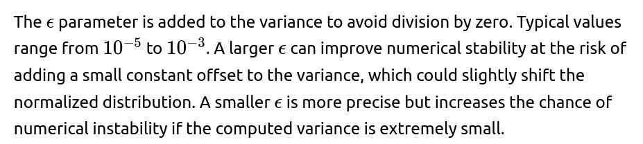
A subtle real-world situation is if you have extremely small feature variance in certain channels. In that case, even a small ϵ might not be enough to keep the denominator from underflowing in lower-precision computations. Empirically tuning ϵ or using dynamic ϵ can sometimes help, but most frameworks’ default is robust enough for a wide range of tasks.

How Should One Debug a Model Where BatchNorm Seems to Work in Training but Fails at Inference?

A classic sign of BN-related inference failure is a big discrepancy between training accuracy and test accuracy. Steps to debug might include:

• Checking that you correctly call model.eval() to freeze BN updates.

• Verifying that the running mean and variance are being properly updated during training. Sometimes a bug prevents them from updating.

• Ensuring that your batch sizes at inference are not zero or extremely small (some libraries treat empty or single-sample batches in an unexpected way).

• Printing out the stored running mean and variance after training to see if they are nonsensical (e.g., infinite or NaN).

• Temporarily forcing the model to use batch statistics even at inference (by staying in train mode) to see if performance matches training. If it does, that means the discrepancy is in the running statistics.

A subtle pitfall is forgetting that certain layers might remain in training mode if the code sets model.eval() incorrectly or only partially. Another issue can be if the data distribution at inference is drastically different, so the “frozen” BN stats are not representative.

That concludes these additional follow-up questions and their detailed answers.