
ML Interview Q Series: Acceptance-Rejection for Half-Normal Distribution Sampling with Exponential Envelope
Browse all the Probability Interview Questions here.
13E-27. Let the random variable Z have the standard normal distribution. Describe how to draw a random observation from |Z| by using the acceptance-rejection method with the envelope density function g(x) = e^(-x). How do you get a random observation from Z when you have simulated a random observation from |Z|?
Short Compact solution
Use acceptance-rejection with envelope g(x) = e^(-x) for x > 0. Specifically:
Generate two independent uniform(0,1) random numbers u1 and u2.
Set y = -ln(u1). This y is a draw from the exponential(1) distribution.
Accept y (and call it v) if u2 <= e^[-(y - 1)²/2]. Otherwise reject and repeat.
Once you have v as a draw from |Z|, generate an independent uniform(0,1) random number u. If u <= 0.5, take Z = v; otherwise take Z = -v.
Comprehensive Explanation
Distribution of |Z|
When Z ~ N(0,1) (standard normal), the random variable |Z| has the following probability density for x > 0:
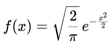
Here x > 0. The factor sqrt(2/pi) ensures that this density integrates to 1 over (0, ∞).
Selecting an Envelope g(x)
We want to sample from f(x) using acceptance-rejection. A common choice for an envelope when x > 0 is the exponential density g(x) = e^(-x), also for x > 0. We just need to find a constant c such that f(x) ≤ c·g(x) for all x > 0.
Computing the Ratio f(x)/g(x)
Consider
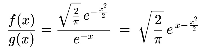
We need the maximum of x - x²/2 over x > 0. By taking the derivative (1 - x) and setting it to zero, we see that the maximum occurs at x=1. Plug x=1 into the above expression:
The exponential factor becomes e^(1 - 1/2) = e^(1/2) = sqrt(e).
Therefore the maximal ratio is sqrt(2/pi) * sqrt(e) = sqrt(2 e / pi).
Hence we set:
Acceptance-Rejection Procedure
Generate from the envelope: Draw X ~ exponential(1), i.e. sample X by taking X = -ln(u1), where u1 is uniform(0,1).
Acceptance check: Generate another uniform(0,1) random number u2. Accept X if
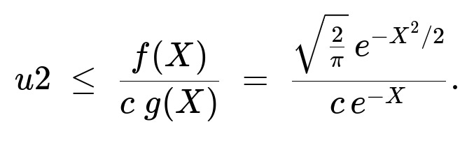
With c chosen as above, this ratio is always ≤ 1. If the acceptance criterion does not hold, reject X and repeat.
Accepted sample: Once accepted, the value of X is distributed according to the density of |Z|. Denote the accepted value by v.
Translating from |Z| to Z
To get a sample from the original standard normal Z, note that Z has equal probability of being positive or negative. So after obtaining v ~ |Z|,
Generate one additional uniform(0,1) random number u.
If u <= 0.5, set Z = v; otherwise set Z = -v.
This ensures that Z has the correct symmetric distribution about 0.
Potential Follow-Up Questions
Why does the exponential(1) distribution serve as a good envelope?
Exponential(1) is often chosen because for x > 0, e^(-x) is a relatively simple function that decays faster than many light-tailed target distributions—like the right half of a normal. It’s straightforward to identify and compute the constant c that bounds f(x)/g(x). Additionally, sampling from the exponential distribution is computationally convenient.
Could we have chosen a different envelope?
Yes. Any g(x) that dominates f(x) on x > 0 with a known inverse transform can be used. However, the constant c might become large if g(x) is a poor match to f(x), which leads to more rejections and less efficiency.
How do we derive the acceptance probability formula in detail?
In acceptance-rejection:
We sample X from g(x) and compute a uniform(0,1) random variable u.
If u <= f(X)/[c*g(X)], we accept X. Otherwise, we reject. This maintains correctness because the expected number of acceptances remains proportional to f(x).
What is the advantage of acceptance-rejection over other methods?
Acceptance-rejection is conceptually simple and easy to apply to many distributions, as long as one can find a suitable envelope g(x). However, if the envelope is not well-fitted or if c is large, the method can be inefficient. Other techniques (like the Ziggurat algorithm for normals, or Metropolis-Hastings in MCMC) might be more efficient in certain scenarios, but acceptance-rejection is often the simplest to illustrate and implement for half-normal sampling.
Could we avoid using acceptance-rejection to generate |Z|?
Certainly. One can generate Z directly from the standard normal via well-known methods (like Box-Muller, or other approaches) and then take the absolute value. The question specifically asks how to do it with acceptance-rejection for educational purposes. In practice, we often just generate Z directly by standard methods and take absolute value when only |Z| is needed.
How do we handle performance concerns in real implementations?
Precomputing constants and storing partial computations helps.
If c is too large (meaning the envelope is a poor fit), the acceptance rate might be low. Then we might pick a better envelope or use another sampling method.
Could this procedure generalize to other distributions beyond the standard normal?
Yes. Acceptance-rejection is a generic technique. As long as you know your target f(x) and can find a tractable envelope g(x) with an easily sampled distribution, you can adapt the same strategy. The key steps are to:
Compute the ratio f(x)/g(x).
Find the maximal value of that ratio over the domain.
Choose c to be that maximum (or slightly larger).
Use uniform draws to accept or reject each sample from g(x).
These points ensure the resulting accepted samples follow f(x).
Below are additional follow-up questions
How do we handle numerical stability if x becomes large and we compute e^(-x^2/2) or e^(-x)?
When x is large, expressions like e^(-x^2/2) or e^(-x) can underflow to 0 in floating-point arithmetic. In an acceptance-rejection context, this can cause the ratio f(x)/[c*g(x)] to incorrectly evaluate to 0 and lead to potential acceptance biases:
A common workaround is to compute log f(x) - log g(x) instead of directly computing e^(-x^2/2)/e^(-x).
You can compute log-ratios safely with built-in log-sum-exp or log-difference-exp functions that handle extremes of floating-point ranges.
After computing the log of the acceptance threshold, compare it with the log of a uniform(0,1) variable (i.e., log(u2)). If log(u2) < [log f(x) - log(c*g(x))], you accept; otherwise, you reject.
This strategy helps avoid any catastrophic underflow and preserves correct acceptance probabilities for large x values.
Could the acceptance-rejection method fail if the maximum of f(x)/g(x) is not correctly identified?
Yes. For acceptance-rejection to work, we need c such that f(x) ≤ cg(x) for all x in the domain. If we mistakenly identify a smaller value for c (perhaps due to a wrong assumption about the maximum of f(x)/g(x)), then there can exist regions where f(x) > cg(x). In that case, some valid x with high target density might always be incorrectly rejected, causing a bias in the samples or the method to fail entirely.
Always ensure that the maximum is computed correctly or that c is chosen conservatively to exceed the true maximum. If necessary, use calculus or numerical optimization to confirm the peak value of the ratio.
What if we cannot analytically find the maximum of f(x)/g(x) for a more complex target distribution?
In some cases, especially for more complicated target densities, finding the exact maximum of f(x)/g(x) analytically might be difficult:
One approach is to use a numerical optimizer or grid search to approximate the maximum.
Another approach is to use an adaptive or iterative scheme that increases c as needed.
If you cannot bracket the maximum precisely but can still find a sufficiently large c to guarantee f(x) ≤ c*g(x), you can proceed. However, an overly large c results in a lower acceptance rate. Balancing these considerations is important to keep the rejection rate reasonable.
How would you adapt this approach if you only want to generate one sample from |Z| and not multiple?
Even if you only need a single sample, the procedure is the same:
Generate a candidate from the envelope (exponential(1) in this case).
Generate a uniform random number for the acceptance check.
Accept or reject. If you reject, you keep repeating. This can be slow if acceptance rates are low. If efficiency is a concern for a one-off sample, you might consider alternative direct methods (like sampling from the normal distribution directly and taking the absolute value).
If we need correlated samples of (|Z|, another variable) can we still use acceptance-rejection?
Acceptance-rejection on its own produces independent samples from |Z|. To produce correlated samples between |Z| and another variable Y, we would need to specify a joint distribution f(|Z|, Y). Simply generating |Z| with acceptance-rejection and then sampling Y from an unrelated procedure does not in general preserve any correlation structure:
One would need the joint density f(|Z|, Y) and an envelope g(x, y) from which you can sample easily.
You could perform acceptance-rejection in multiple dimensions if the ratio f(x, y)/g(x, y) is tractable.
Alternatively, you might adopt an MCMC technique, such as a Metropolis-Hastings sampler, to sample from the joint distribution more directly.
Are there any special considerations if we want to implement the method on hardware with limited precision, like certain embedded systems or GPUs?
Limited precision environments may exacerbate underflow/overflow issues:
You might need to store relevant constants (like c) in higher precision data types or keep them in log form to preserve accuracy.
The calculation of exponentials might require specialized functions (e.g., approximate hardware instructions or table lookups).
Ensuring a stable and correctly seeded pseudo-random number generator is also important, as repeated patterns in uniform draws can bias the acceptance-rejection process. In practice, these complexities can be mitigated by carefully tested libraries optimized for the specific hardware environment.
How does the acceptance rate influence whether this method is practical in a high-throughput environment?
The acceptance rate is the average probability that a proposed sample is accepted. If the ratio f(x)/[c*g(x)] is often very small, many candidates will be rejected:
A low acceptance rate means more computational effort per accepted sample. This can be problematic when generating millions of samples in real-time or in large-scale simulations.
Even for standard normal distributions, acceptance rates may be acceptable with a well-chosen envelope, but for certain heavy-tailed or complex distributions, acceptance-rejection can become inefficient.
Profiling your sampler to measure actual acceptance rates is critical for deciding if acceptance-rejection is the right approach in a production setting. If it is too slow, consider alternative sampling methods (e.g., specialized algorithms for normal or half-normal distributions, or other advanced sampling techniques like importance sampling or MCMC).
What if you need to generate both positive and negative samples from the normal, but with different probabilities (i.e., not 50/50)?
The standard normal is symmetric, so typically Z is equally likely to be positive or negative. However, if you had a custom scenario where the sign distribution was not 50/50:
You cannot simply flip the sign with a 0.5 threshold. Instead, you need a different logic that chooses signs according to your desired proportion p for positive vs. 1-p for negative.
If p is not 0.5, the resulting distribution is no longer a standard normal. It becomes a “folded-shifted” distribution if the absolute value is still normal-like.
In that case, you should revisit the target distribution definition and potentially redo the acceptance-rejection logic for that specific asymmetric distribution if needed.