ML Interview Q Series: Achieving Probabilistic Multi-Class Classification with Softmax and Cross-Entropy

📚 Browse the full ML Interview series here.

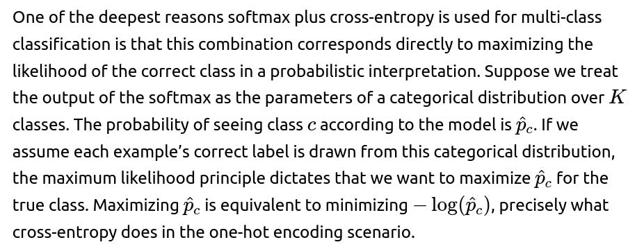
Softmax and Cross-Entropy: Write the formula for the softmax function for a $K$-class classification problem. Using a softmax output, define the cross-entropy loss for a single training example. Explain why the softmax + cross-entropy combination is a natural choice for multi-class classification (hint: probabilistic interpretation and connection to maximum likelihood).

Understanding the Softmax Function

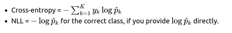
Cross-Entropy Loss for a Single Example

Why Softmax + Cross-Entropy Is a Natural Choice for Multi-Class Classification

Another way to see it is that cross-entropy quantifies the distance between two probability distributions: the true distribution (one-hot) and the predicted distribution (softmax output). Minimizing cross-entropy is then a direct measure of how well the predicted distribution matches the ground truth.

From a practical training perspective, gradients derived from the cross-entropy loss with respect to logits are typically well behaved, leading to stable and efficient training. Softmax ensures the outputs are positive and sum to 1, aligning well with the notion of class probabilities, while cross-entropy enforces that the predicted probability for the correct class should be as high as possible.

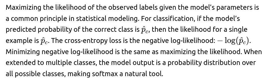
Maximum Likelihood Connection

Detailed Explanations and Possible Interview Follow-up Questions

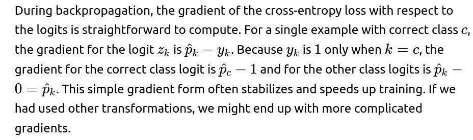
How Does the Softmax Transform Help with Gradient Computations?

A subtlety is that an implementation that first computes softmax and then applies cross-entropy might face numerical instability if done naively. However, modern libraries combine these two steps into a single “log-softmax + negative log-likelihood” operation that is numerically stable (for instance, in PyTorch, it is often implemented as torch.nn.CrossEntropyLoss, which handles the logits directly).

Why Not Use Mean Squared Error for Multi-Class Classification?

Mean squared error (MSE) can be used for classification in principle, but it is typically discouraged. If we place an MSE loss on the raw logits versus a one-hot target, the resulting gradient can be much less direct in driving the correct class probability to 1 and the other probabilities to 0. The probabilistic interpretation is also less direct with MSE, and the gradients can suffer from slower convergence. Cross-entropy directly corresponds to maximizing the log-likelihood of the correct class. This alignment to probability theory tends to give better and faster convergence in practice.

Are There Numerical Stability Concerns with Softmax + Cross-Entropy?

Directly exponentiating large logits can produce extremely large values, leading to floating-point overflow. Similarly, log⁡ of very small probabilities can underflow. This can be partially alleviated by subtracting the maximum logit from all logits before exponentiating, which is a common trick for numerical stability. For cross-entropy, deep learning libraries will often combine the log-softmax operation with the negative log-likelihood operation in a single function. This ensures stable gradient computations even for large or small logits.

Could You Show a Simple PyTorch Code Snippet for Training a Model with Softmax and Cross-Entropy?

Below is a short example that demonstrates how you might use PyTorch with cross-entropy loss for a multi-class classification model. Notice that we do not manually apply a softmax layer when using torch.nn.CrossEntropyLoss; PyTorch’s cross-entropy function expects raw logits and handles the log-softmax operation internally.

import torch
import torch.nn as nn
import torch.optim as optim

# Suppose we have a simple feedforward network for K-class classification
class SimpleClassifier(nn.Module):
    def __init__(self, input_dim, hidden_dim, num_classes):
        super(SimpleClassifier, self).__init__()
        self.fc1 = nn.Linear(input_dim, hidden_dim)
        self.relu = nn.ReLU()
        self.fc2 = nn.Linear(hidden_dim, num_classes)

    def forward(self, x):
        # Returns raw logits
        x = self.fc1(x)
        x = self.relu(x)
        x = self.fc2(x)
        return x  # Softmax is internally handled by cross_entropy loss

# Create model, define loss and optimizer
model = SimpleClassifier(input_dim=10, hidden_dim=20, num_classes=5)
criterion = nn.CrossEntropyLoss()  # Expects raw logits
optimizer = optim.SGD(model.parameters(), lr=0.01)

# Dummy data for demonstration
x_train = torch.randn(8, 10)         # batch of size 8, input_dim=10
y_train = torch.randint(0, 5, (8,))  # class labels from 0 to 4 for 8 examples

# Forward pass
logits = model(x_train)
loss = criterion(logits, y_train)

# Backward pass
optimizer.zero_grad()
loss.backward()
optimizer.step()

In this snippet, the final layer output is raw logits. The function nn.CrossEntropyLoss internally applies softmax and computes cross-entropy. The backpropagation step calculates the gradients and updates the weights to maximize the log probability of the correct classes.

How Can We Interpret the Outputs?

After training, when you apply the model to new data, you typically take the output logits and pass them through F.softmax(logits, dim=1). This yields a probability distribution over the K classes. You can then pick the class with the highest probability as your prediction. Alternatively, some frameworks just let you call logits.argmax(dim=1) to get the predicted class index directly.

What If We Have Imbalanced Classes?

Cross-entropy can be adapted to handle class imbalance by weighting certain classes more heavily. In PyTorch, this can be achieved by passing a weight argument to the CrossEntropyLoss constructor, where the weight is often chosen inversely proportional to the frequency of each class. Another approach is focal loss, which modifies cross-entropy to emphasize hard-to-classify examples. Softmax itself remains the same (since it is simply turning logits into normalized probabilities), but the loss function can be adapted to focus on classes that are underrepresented.

Is There a Direct Connection to Logistic Regression in the Binary Case?

Could You Summarize the Key Takeaways Without Repetition?

Softmax transforms logits into probabilities. Cross-entropy quantifies how well those probabilities match the one-hot ground truth. Minimizing cross-entropy is equivalent to maximizing the likelihood of the correct class. This alignment with probability theory leads to stable training, straightforward gradient computations, and better interpretability in real-world classification tasks.

---

Below are additional follow-up questions

How does multi-label classification differ from multi-class classification when using softmax and cross-entropy, and what are the main pitfalls?

In a multi-class setting, each instance belongs to exactly one of the K classes. The softmax layer outputs a probability distribution over these K classes, and we typically use cross-entropy to evaluate the model’s correctness in picking one dominant class per example.

In a multi-label setting, each instance can have multiple valid labels simultaneously. Using a softmax across K classes forces these probabilities to sum to 1, which is a conceptual mismatch for multi-label scenarios. Instead, we usually apply an independent sigmoid function to each of the K outputs and then use binary cross-entropy for each label separately.

Pitfalls or edge cases:

• If multi-label data is incorrectly modeled with a softmax output layer, the model is forced to rank classes against each other, preventing it from learning that multiple labels can be correct at once.

• During real-world collection, we might have incomplete labels. Some relevant labels could be missing due to annotation errors, which can confuse training if we treat them as negatives. Care must be taken to ensure data quality or to employ partial-label or weakly supervised learning strategies.

• If the number of potential labels per example is large, the model might incorrectly focus on the most frequent label combinations, missing rare but critical label co-occurrences.

How do label noise or uncertain labels impact the softmax + cross-entropy approach, and what can be done to mitigate issues?

Label noise occurs when some training samples have incorrect or ambiguous labels. This can cause cross-entropy to push the model aggressively toward the wrong target distribution.

To mitigate:

• Label smoothing: This modifies the one-hot targets so that they are not strictly 0 or 1 but slightly softer. This approach can help the model become less overconfident and more robust to minor label errors.

• Data cleaning and validation: Sometimes the best approach is to filter out or correct problematic samples.

• Loss function variants: Some robust loss functions (e.g., symmetric cross-entropy or focal loss) can down-weight or handle incorrect labels better by not punishing certain errors as harshly.

• Uncertainty modeling: One can model uncertain labels through probabilistic label representations (for example, 0.7 for class A, 0.3 for class B if the true label is ambiguous). This is more involved than standard cross-entropy but can yield a better representation of real-world uncertainty.

Pitfalls or edge cases:

• Overfitting to noisy labels can cause the model to memorize incorrect training targets, resulting in poor generalization.

• A small fraction of label noise can dramatically increase training time if the model tries to reconcile conflicting labels. Early stopping or careful learning rate scheduling may help.

• Overly aggressive label smoothing can obscure valid signals and degrade performance.

What is label smoothing in cross-entropy, and how does it impact the training process?

Motivation:

• Reduces overfitting by preventing the model from becoming overconfident (where predicted probabilities are extremely close to 1 or 0).

• Helps the model learn more generalizable representations.

Pitfalls or edge cases:

• In extremely imbalanced classification problems, label smoothing might need further adjustment so that underrepresented classes are not overly penalized.

• Some interpretability methods might become less direct if the final predicted probabilities are influenced by label smoothing.

How do we interpret softmax outputs for out-of-distribution (OOD) samples, and what pitfalls might arise?

Softmax outputs can be misleadingly high for OOD inputs. Even if the input is entirely unlike any training sample, the softmax forces a probability distribution over the known classes, potentially giving a false sense of confidence.

Pitfalls:

• In safety-critical applications (like autonomous driving or medical diagnosis), high-confidence wrong predictions on OOD data can be dangerous.

• A model might assign a near-1 probability to a random foreign image simply because it aligns in certain uninformative ways with the training data.

Potential solutions:

• Out-of-distribution detection using specialized metrics (e.g., Mahalanobis distance, confidence calibration, or separate OOD classifiers).

• Temperature scaling or Monte Carlo dropout to better calibrate probabilities.

• Ensemble methods that can provide additional signals for uncertainty if an example is outside of the training distribution.

Why might a model become overconfident with softmax, and how can this be addressed?

Softmax can produce a “winner-takes-all” effect, where the highest logit leads to a probability close to 1. Deep neural networks are especially prone to overconfidence if they are trained to minimize cross-entropy without additional regularization.

Methods to address overconfidence:

• Calibration techniques: Such as Platt scaling or temperature scaling. Temperature scaling modifies the logits before softmax by dividing by a learned temperature parameter, which can spread out or compress the distribution.

• Label smoothing: As discussed, it reduces the gap between perfect confidence and smaller probabilities, discouraging overconfidence.

• Ensemble approaches: Combining multiple models or using Bayesian neural network approximations can produce more conservative posterior estimates.

• Confidence penalization: Some specialized losses directly penalize confident outputs when they are incorrect.

Pitfalls or edge cases:

• Overconfident outputs might remain if the training data is small, extremely noisy, or highly imbalanced.

• Some calibration methods might degrade accuracy if not applied properly (for example, an over-aggressive temperature scaling might flatten the distribution too much and make predictions less discriminative).

What techniques can be applied for a large number of classes to speed up training with softmax and cross-entropy?

When K is very large (e.g., tens or hundreds of thousands of classes), computing a full softmax can be computationally expensive.

Potential techniques:

• Hierarchical softmax: Decompose the output layer into a tree-based structure, reducing computation to a path of smaller softmax operations.

• Sampling-based methods: Such as negative sampling or importance sampling. We only sample a subset of negative classes during each gradient update instead of all K classes.

• Approximate methods: Like candidate sampling (similar to negative sampling), or using specialized GPU kernels that are optimized for large vocabulary tasks (e.g., large vocabulary language modeling).

Pitfalls or edge cases:

• Hierarchical softmax might complicate training because constructing an optimal tree structure can be non-trivial. A suboptimal tree might slow down convergence or reduce final accuracy.

• Sampling methods must be carefully designed to ensure the sampled negatives reflect the overall distribution. Poor sampling strategies can bias parameter updates.

• Debugging or validating probabilities can be harder with approximate methods since the reported softmax probabilities might not strictly sum to 1 over the entire class set.

Are there alternatives to cross-entropy for multi-class tasks, and when might they be beneficial?

Yes, there are alternative loss functions:

• Focal loss: Places more emphasis on hard or misclassified examples, often used for handling class imbalance or tasks where some samples are especially critical.

• Squared error loss: Rarely used in multi-class classification because it can lead to slower convergence and less direct gradient signals.

• Contrastive losses: In some metric learning contexts, you train an embedding rather than a classifier, though eventually a softmax-like step might still be used for final classification.

• Label-distribution-aware margin (LDAM) loss: Addresses class-imbalance by adjusting margins for minority vs. majority classes.

Pitfalls or edge cases:

• Focal loss hyperparameters (like the focusing parameter γ) must be carefully tuned; if set incorrectly, the model can over-focus on certain examples.

• Some specialized losses might not be as straightforward to optimize at large scale compared to cross-entropy.

• Certain alternative losses break the neat probabilistic interpretation that cross-entropy + softmax provides, making post-hoc probability calibration or interpretability trickier.

How are the final layer’s weights and biases typically initialized, and what effect does this have on softmax?

In many deep learning frameworks, the final linear (fully connected) layer that outputs logits is often randomly initialized with something like Xavier (Glorot) or Kaiming (He) initialization. The bias terms often start at zero or a small constant.

Effects:

• Proper initialization helps preserve gradient flow, preventing vanishing or exploding gradients through earlier layers.

• If weights are initialized too large, the logits might start out with large magnitudes, which can produce saturated softmax probabilities, making learning slow in the early stages.

• Some practitioners initialize the final layer bias toward negative values to prevent saturating the softmax or to ensure the initial predictions are “uncertain.”

Pitfalls or edge cases:

• If K is huge, and each logit is given a wide distribution at initialization, you can end up with numerical overflow or “spiky” probabilities in the first few training steps.

• Improper initialization might cause the model to get stuck in local minima or lead to degenerate solutions if combined with certain regularization schemes.

What is the difference between cross-entropy and negative log-likelihood (NLL) in frameworks like PyTorch?

In PyTorch:

• CrossEntropyLoss typically expects raw logits. It then applies a log-softmax internally and computes the negative log-likelihood loss.

• NLLLoss expects log probabilities as inputs. You must manually apply log-softmax on the logits before passing them to NLLLoss.

Conceptually, cross-entropy and negative log-likelihood are extremely similar. The only difference in typical usage is that cross-entropy includes the softmax step internally, while NLL expects pre-log-softmax probabilities. The underlying math is the same:

Pitfalls or edge cases:

• Passing logits directly to NLLLoss without applying log-softmax will result in incorrect losses.

• Numerically, combining softmax and cross-entropy in one step (i.e., using CrossEntropyLoss) is typically more stable because it can manage large or small logits internally.

In what scenarios might you interpret logits directly instead of using the softmax probabilities?

Sometimes you want to analyze the relative scores rather than the normalized distribution:

• Margin-based tasks: In certain metric learning setups or in SVM-like approaches, the margin between logits can matter more than their normalized probabilities.

• Uncertainty methods: Some out-of-distribution detection strategies look at logit magnitudes or pairwise logit differences.

• Teacher forcing or knowledge distillation: You might want the teacher model’s logits to remain unnormalized when transferring knowledge to the student model. Though typically, “soft targets” are used via a temperature-scaled softmax, sometimes direct logit-level supervision is also considered.

Pitfalls or edge cases:

• Logits can be very large or small, so interpreting them alone can be less intuitive than looking at a probability distribution.

• Directly comparing logits across different input samples can be problematic if the network’s overall scale of logits shifts over time or if there’s no consistent reference point.

• If you rely purely on logits without normalizing, you lose the straightforward probabilistic interpretation that can be important in many real-world decision pipelines.

Below are additional follow-up questions

Could you discuss how softmax behaves when there are extremely large numbers of classes, and what practical strategies exist to deal with the computational challenges?

When the number of classes K is extremely large (e.g., vocabulary size in natural language tasks reaching tens or hundreds of thousands), computing the softmax denominator

becomes costly, both in time and memory. The exponentiations scale linearly with K, and this cost can be prohibitive in real-world systems with limited GPU/CPU memory.

One common strategy to mitigate this is the use of hierarchical softmax, which places labels into a tree structure. Instead of computing exponentials for all K classes simultaneously, you break down the softmax computation into a sequence of smaller softmaxes along the path from the tree’s root to a leaf (the leaf corresponds to a specific class). This reduces complexity from

O(K)

to around

O(log⁡K)

in many practical setups.

Another strategy is to use negative sampling (particularly popular in word embedding training for large vocabularies). Rather than normalizing across all K classes, you sample a small number of “negative” classes each batch. This is not a perfect approximation, but it often suffices, especially in language modeling or recommender systems, providing a more scalable approach to training models where K is massive.

Edge cases or pitfalls:

• Hierarchical softmax depends on how you build the class hierarchy. A poorly designed tree (e.g., unbalanced structure) might degrade performance and not yield the expected savings.

• Negative sampling modifies the training objective slightly, possibly introducing a mismatch between training and true log-likelihood. This can lead to suboptimal probabilities if you truly need accurate probabilities over the entire label space.

How does softmax behave under the presence of out-of-distribution inputs, and how might this impact the reliability of predicted probabilities?

Softmax will always produce a valid probability distribution over the K classes, even for inputs that do not resemble anything in the training set (out-of-distribution samples). Because of the exponential in the numerator, a single logit that is relatively higher than the others can lead to a near-1 predicted probability for a class, even if the input is something the model has never been trained on or does not understand.

This can generate overconfident predictions on out-of-distribution data. A model may produce a probability close to 1 for a class, misleading the user into believing that the model is certain. In reality, the model simply does not have a mechanism to say “none of the above.”

Strategies to address this include:

• Calibration methods such as temperature scaling, where you introduce a scalar temperature

  T

  into the softmax:

• A higher temperature can reduce overconfidence by flattening the distribution.

• Out-of-distribution detection algorithms, such as using the magnitude of feature embeddings or specialized uncertainty models (e.g., Bayesian neural networks, ensembles, or explicit out-of-distribution detectors).

Pitfalls or edge cases:

• Merely tuning temperature can make the model less certain across all inputs, including in-distribution data. This uniform flattening can degrade performance if not carefully validated.

• True out-of-distribution detection typically requires separate modeling or side-information. Simply using softmax probabilities can be misleading.

Could you explain what happens when training data contains label errors, and how softmax cross-entropy might exacerbate or mitigate issues with noisy labels?

When training data contains mislabeled examples, the cross-entropy loss penalizes the model for not predicting those (incorrect) labels with high probability. Because the model is forced to fit possibly contradictory or impossible targets, it can lead to overfitting to noise. Softmax cross-entropy strongly pushes the model to output high probability for the presumably correct class, so if that label is actually incorrect, the model’s parameters may shift in a way that hurts overall generalization.

Possible mitigation strategies include:

• Label smoothing. Instead of a hard 1 for the correct class, you distribute a small portion of probability across the other classes. This reduces the penalty for not matching the “true” label exactly, thereby softening the impact of noise.

• Data cleaning or automated relabeling. If there is a systematic pattern to label noise, you might train a small model or use heuristics to identify and correct mislabeled samples.

• Robust loss functions like the symmetric cross-entropy or bootstrap losses. These can handle some fraction of noisy labels better than standard cross-entropy.

Pitfalls or edge cases:

• Label smoothing can harm legitimate certainty if your data is actually clean and the model is capable of near-perfect classification. You must weigh the trade-off of potentially reduced overfitting vs. slightly decreased peak accuracy.

• Methods like symmetrical cross-entropy are not widely implemented in standard libraries, so you may need a custom implementation and thorough experiments to verify gains in the presence of label noise.

In practice, how can we handle scenarios where multiple classes can be correct (multi-label classification) if we only have access to softmax and cross-entropy tools?

Standard softmax cross-entropy is premised on exactly one correct class per example. If an example can legitimately belong to multiple classes simultaneously (e.g., in image tagging where a single image might contain a cat, a dog, and a tree), softmax is not appropriate.

Instead, a common approach is to have a separate sigmoid output unit per class, turning the problem into multiple independent binary classification tasks. Each class’s membership is predicted via

and you use binary cross-entropy loss for each class:

Pitfalls or edge cases:

• Some tasks might still have correlation among labels (e.g., if “car” is present, “road” might have higher likelihood). Independent sigmoid predictions ignore these correlations. More sophisticated multi-label methods might use structured approaches or additional regularizers to account for label dependencies.

• The magnitude of the output for each class is not constrained to sum to 1. This is correct for multi-label classification but can lead to different interpretive pitfalls (e.g., your probabilities can collectively sum to a value greater than 1).

Could you address how softmax cross-entropy loss behaves when data is highly imbalanced among classes?

In highly imbalanced multi-class classification, some classes might be significantly underrepresented. Standard softmax cross-entropy treats each class equally, so the network may learn to ignore rare classes, because guessing frequent classes might minimize loss on the majority of data.

Practical remedies include:

• Class weighting. Multiply the cross-entropy terms by a weight inversely proportional to class frequency. This ensures that mistakes on rare classes are penalized more heavily, encouraging the model to pay attention.

• Oversampling. Repeatedly sample examples from minority classes so that they appear more often during training, or use synthetic data generation techniques (e.g., SMOTE in certain contexts).

• Focal loss. Although introduced for object detection tasks, it adjusts the cross-entropy to focus more on misclassified examples, which can help with class imbalance.

Pitfalls or edge cases:

• Overweighting minority classes can cause the model to overfit those classes if the data is too scarce or noisy. You might start seeing many false positives in the rare class.

• Synthetic oversampling can introduce data artifacts or reduce diversity if not done carefully.

How do we interpret the loss landscape for cross-entropy, and are there optimization concerns specific to softmax cross-entropy that might not arise in other loss functions?

Cross-entropy loss combined with softmax has a particular geometry that can be steeper (in gradient terms) when the model’s probability for the true class is low, and shallower when the model is confident and correct. This typically yields fast correction of large errors and stable convergence when the model is near a good solution.

Potential optimization concerns:

• Vanishing or exploding gradients can still happen if logits are extremely large (positive or negative). Implementations with the log-sum-exp trick mitigate most numeric instability, but extreme parameter initializations or poorly tuned learning rates can still cause issues.

• Local minima or saddle points are generally less of a concern in very high-dimensional neural networks. Empirically, we often find “good enough” minima. However, cross-entropy doesn’t necessarily guarantee we find the global best minimum, only that we keep pushing probabilities to match the data distribution.

Pitfalls or edge cases:

• Poor initialization can cause a model to get “stuck” if it’s extremely biased toward certain classes early on. Carefully chosen initialization or batch normalization helps.

• If your data is extremely easy and the model is very high capacity, cross-entropy can approach near-zero on training data, risking overfitting if not controlled with regularization or early stopping.

What is label imbalance vs. class imbalance, and how do they each affect the cross-entropy training dynamic?

Class imbalance refers to some classes having far more samples than others. Label imbalance can also appear in multi-label settings (where certain classes are less likely to appear together). In single-label classification, “label imbalance” and “class imbalance” are effectively the same.

When a model is trained with standard cross-entropy on highly imbalanced data, the major classes dominate the training signal. The model might learn to classify everything as the majority class, yielding good average accuracy if that class is indeed the majority. Cross-entropy will not inherently fix this unless we adjust the training procedure (class weighting, oversampling, etc.).

Pitfalls or edge cases:

• Sometimes data imbalance is a true reflection of real-world frequencies. Over-correcting can produce artificially balanced predictions that harm performance metrics such as precision or false positive rate for the minority classes.

• Splitting your dataset into train/validation/test might preserve overall distribution, but you might end up with extremely few examples of minority classes in the test set, leading to high variance estimates of model performance for those classes.

Could you describe how soft labels differ from one-hot labels in training, and what consequences arise when using softmax plus cross-entropy on soft labels?

Soft labels refer to the case when the true label distribution is not a strict one-hot vector but rather a probability distribution (e.g., there is a 70% chance the image is a cat, 30% chance it is a fox). Softmax cross-entropy can seamlessly incorporate these distributions:

where now

is not 0 or 1 but can lie in [0,1]. Minimizing cross-entropy encourages the model to match its predicted distribution

to the target distribution

Such an approach arises in knowledge distillation, where a teacher model provides “soft” targets to a student model. The teacher’s output distribution can contain valuable relative probability information about classes beyond the single top label.

Edge cases or pitfalls:

• If the soft labels come from an imperfect teacher or approximations, the student can inherit these mistakes or biases.

• The distribution might not be truly representative of the underlying data, especially if teacher calibration is poor. This can harm final performance on real data with crisp labels.

In the context of modern large-scale models, how do gradient-based optimization behaviors differ between cross-entropy and alternative losses?

Cross-entropy typically produces gradients that are well-scaled for classification tasks, leading to stable training even for large neural networks. Some alternative losses (like hinge loss or squared error) can lead to slower training convergence or less intuitive probability outputs. Cross-entropy’s gradient is:

which is linear in the difference between predicted and target probability. This yields strong directional signals even for small mismatches, helping large-scale models converge quickly. By contrast, hinge loss has zero gradient once a margin is satisfied, which can lead to less fine-grained tuning after that point.

Pitfalls or edge cases:

• Large-scale models can still get stuck due to improper learning rates. If the learning rate is too high, the gradient from cross-entropy can cause instability or diverging loss.

• Cross-entropy presumes that each sample belongs to one class with high certainty (barring label smoothing), which might not perfectly match real-world uncertainty.

Could you clarify the role of temperature scaling in both training and inference phases, and how it affects cross-entropy optimization?

Temperature scaling, using a temperature

T

in the softmax,

can serve two distinct purposes:

1. During training: A higher temperature can make the distribution softer. This is sometimes used in knowledge distillation, where the teacher’s output is softened so that the student can learn from relative probabilities across classes.

2. During inference or calibration: If a model is overconfident, scaling up the temperature

   T>1

can flatten predictions, improving calibration metrics while usually maintaining the same argmax class. Conversely,

T<1

sharpens the distribution, making the model more confident.

Pitfalls or edge cases:

• Temperature is typically not learned end-to-end in standard training. If you freeze model weights and only optimize for temperature post-hoc on a validation set, you risk mismatch between training and inference objectives.

• Overusing a high temperature can degrade model accuracy if the highest predicted probability gets pulled too close to the others, causing more confusion among plausible classes.

When would it be useful to inspect per-class cross-entropy, and how might that help in debugging model issues?

Inspecting per-class cross-entropy means computing:

focusing on how well the model handles data points belonging to class k. This can reveal whether the model struggles to separate that specific class from others. For instance, if you see that a particular class has a significantly higher average cross-entropy than others, the model may not have learned distinctive features to correctly classify that class.

This can be especially useful in debugging:

• Class imbalance: Maybe that class is underrepresented, and the model cannot confidently assign it.

• Data quality: Possibly the data for that class is noisier or contains mislabeled examples.

• Inherent difficulty: It may simply be a more challenging class to learn (e.g., visually subtle differences).

Pitfalls or edge cases:

• Looking at per-class cross-entropy only helps if you have enough data points per class. If a class is extremely rare, your estimates of

  

  might be noisy.

• It can be time-consuming to break down the loss at this level for large datasets. Usually, a single average cross-entropy is monitored, but occasionally you might sample subsets for deeper debugging.

Could you expand on using cross-entropy plus auxiliary losses, and how such multi-task or auxiliary training setups might affect the softmax output?

In deep models, especially in multi-task learning or architectures like Inception networks, you sometimes add auxiliary classification heads, each with its own cross-entropy loss. You combine these cross-entropies (often with different weighting) into a final scalar loss. The rationale is that these auxiliary heads provide additional gradient signals at intermediate layers, stabilizing training and improving feature representations.

For instance, in some networks, an auxiliary head is attached mid-network to output class predictions at an earlier stage. This partial network cross-entropy can help with vanishing gradients or guide early layers to learn better discriminative features.

Pitfalls or edge cases:

• Balancing loss weights is tricky. If the auxiliary loss is too strongly weighted, the main objective might degrade. If it’s too weak, you might not see the intended benefit.

• Additional heads can introduce overhead. At inference time, you often ignore them, but they still add complexity during training and require memory.

What if we want to modify the loss function to penalize incorrect classifications unevenly across classes? How does that interact with softmax and cross-entropy?

Softmax cross-entropy can be adapted by incorporating class-dependent costs. Specifically, you can multiply each term in the cross-entropy sum by a class weight

Here, classes with higher

produce a larger contribution to the loss if incorrectly classified, compelling the model to pay closer attention. This approach is standard for dealing with class imbalance or when certain misclassification errors are particularly costly in the real world.

Pitfalls or edge cases:

• Determining

  

  might require domain knowledge or empirical tuning. Arbitrarily large weights can destabilize training, as the gradient might become very large for minority classes.

• If the dataset distribution changes over time (non-stationary environments), fixed class weights might become outdated and harm performance.

How can we differentiate between optimizing accuracy vs. optimizing cross-entropy, and are there cases where these objectives diverge?

Minimizing cross-entropy is equivalent to maximizing the likelihood of the data under the model’s predictions, and in a standard single-label classification scenario, it often correlates with improved accuracy. However, cross-entropy is more fine-grained. If a model incorrectly classifies an example, the loss punishes the severity of that misclassification based on how probable it considered the correct label.

A model could theoretically have a high accuracy but still give poor probability estimates for some examples. Meanwhile, a different model might produce better calibrated probabilities (lower cross-entropy) but the same or slightly lower accuracy. In some domains, having well-calibrated probabilities is more critical than raw accuracy (e.g., medical diagnoses, risk assessment).

Pitfalls or edge cases:

• In a competitive environment, maximizing accuracy on a test set might overshadow the importance of well-calibrated probabilities. This can be detrimental in risk-sensitive applications.

• Thresholding for classification (e.g., deciding a class if probability > 0.5) might yield suboptimal accuracy if class distribution is skewed. Adjusting that threshold after training can maximize accuracy without necessarily altering cross-entropy.

What is the intuition behind combining or regularization with cross-entropy, and how does it help prevent overfitting?

Regularization techniques (e.g., weight decay with an norm) add a penalty term to the overall loss, typically

where

are model parameters. This penalty encourages smaller parameter magnitudes, reducing overfitting by limiting how drastically the model can assign large positive or negative logits to certain classes. It works in tandem with cross-entropy:

Cross-entropy alone focuses on fitting the labels precisely, and can lead to large weights that push the correct class probabilities near 1. The regularization dampens extreme weight updates, leading to better generalization.

Pitfalls or edge cases:

• Over-regularization can hamper the model from capturing genuine complexities in the data, leading to underfitting.

• The tuning of

  λ

  is critical and typically validated via experiments on a hold-out set. If not carefully chosen, the benefits of cross-entropy can be overshadowed by the penalty term.

Could you discuss how training dynamics might differ if the model outputs logits in different numeric ranges, and does softmax cross-entropy inherently adapt to that?

The softmax function depends on relative differences in logits. If we have logits

, adding a constant

c

to all logits doesn't change the softmax probabilities because:

However, large magnitude differences among logits can still affect numeric stability. The cross-entropy itself adapts to the relative scale of logits, but at an extreme scale (very large or very small logits), floating-point overflow or underflow can occur without a stable implementation.

Pitfalls or edge cases:

• If your model’s architecture or initialization systematically produces extremely large logits, you risk numerical instability. While libraries mitigate this with log-sum-exp, excessively large values can still degrade gradient precision.

• In practice, batch normalization or carefully chosen initializations help keep logits in a more moderate range for stable training.

What approach might you take if you realize that the cross-entropy metric on training data continues to decrease, but your validation cross-entropy has plateaued or started increasing?

This scenario typically indicates overfitting. The model is continuing to fit the idiosyncrasies of the training set but not improving (and possibly worsening) on unseen data.

Common remedies:

• Early stopping: Stop training once validation loss no longer improves.

• Stronger regularization: Add or increase weight decay, dropout, or data augmentation.

• Data augmentation: Enrich the training data distribution so that the model generalizes better.

• Adjusting hyperparameters: A smaller learning rate or modified batch size can sometimes stabilize generalization.

Pitfalls or edge cases:

• Overfitting might be mild, and a small rise in validation cross-entropy might still correspond to improved accuracy if the distribution of predictions is shifting. Monitor multiple metrics.

• If the dataset is too small or not representative, no standard method might suffice; collecting more data is often the most impactful approach.

Could you elaborate on the relationship between cross-entropy and perplexity, especially in language modeling?

Perplexity is a commonly used metric for language models, defined as

where cross-entropy is typically measured in nats or bits, depending on the log base. In practice, it’s measured per token. Minimizing cross-entropy directly leads to minimizing perplexity. A lower perplexity indicates that the model is assigning higher probability to the correct next token.

Pitfalls or edge cases:

• Perplexity can be misleading if the dataset has significant noise or if the model memorizes training data, artificially inflating performance on a small validation set.

• Large vocabulary sizes compound the difficulty of computing perplexity precisely. That’s why techniques like hierarchical softmax or sampling-based approximations are used in large-scale language modeling.

How does label smoothing compare to knowledge distillation, given they both provide a softer target distribution?

Label smoothing is a simple technique that replaces the hard one-hot target with a distribution that’s mostly on the correct class but allocates a small fraction across other classes. Knowledge distillation, on the other hand, uses the entire output distribution (logits or softmax probabilities) of a teacher model. This can carry more nuanced information—for instance, the teacher might assign a small but distinct probability to semantically similar classes.

Both reduce the model’s tendency to become overconfident. However, label smoothing is a uniform “softness,” while knowledge distillation is structured “softness” informed by the teacher’s predictions.

Pitfalls or edge cases:

• If the teacher model is poorly calibrated or has biases, the student inherits these biases.

• Label smoothing does not incorporate any semantic relationships across classes, so it may not be as beneficial if you want the model to learn those nuanced relationships.

In situations with budget constraints for training time, how can we speed up convergence with cross-entropy, and what trade-offs might arise?

Cross-entropy typically converges quickly given well-tuned hyperparameters, but in large-scale problems you might still need to accelerate training. Techniques include:

• Mixed precision or half-precision training: Reduces memory bandwidth, can speed up matrix operations on modern GPUs.

• Gradient accumulation or large-batch training: If you have enough GPU memory or across distributed systems, you can increase batch size to make full use of hardware parallelism.

• Learning rate scheduling: Cyclical or warm restarts can help find faster convergence paths.

Potential trade-offs:

• Large batch sizes can degrade generalization by reducing the stochasticity in gradient estimates, potentially leading to sharper minima.

• Mixed precision can introduce numerical issues if not implemented carefully, especially for the logits or the log-sum-exp part of softmax. Most frameworks handle this gracefully, but overflow can still occur if logits are extremely large.