ML Interview Q Series: Addressing Correlated Predictors (Multicollinearity) in Regression using Regularization and PCA.

📚 Browse the full ML Interview series here.

Say you are running a multiple linear regression and believe there are several predictors that are correlated. How will the results of the regression be affected if they are indeed correlated? How would you deal with this problem?

This problem was asked by Google.

Understanding how correlated predictors (also known as multicollinearity) affect multiple linear regression is crucial for both the interpretation of the model and for ensuring that the model’s parameters can be reliably estimated. Correlated predictors can cause instability in coefficient estimates, potentially inflating their variance and making it difficult to interpret which predictors are truly driving changes in the response. Below is a detailed discussion of what happens when predictors are correlated, why it is a problem, and how it can be handled in practice.

Deeper Explanation of Multicollinearity

When two or more predictors are highly correlated, the design matrix used in linear regression will have less “independent” information. In multiple linear regression, we typically assume a model of the form:

Interpretation Challenges

In a scenario of multicollinearity:

• The confidence intervals for some coefficients can become very wide, making it less clear whether the predictor is truly significant.

• Coefficients may change drastically if you add or remove a correlated predictor.

• The magnitude and sometimes even the sign of correlated predictors’ coefficients can shift in unpredictable ways.

Predictive vs. Interpretive Goals

If your main objective is purely predictive, having correlated predictors is often less of a problem—your model may still produce good predictions. However, if you need interpretability (for instance, understanding which variables have the strongest influence on the response), high correlation among predictors can obscure which factors are actually important.

Dealing with the Problem

Domain Knowledge to Remove or Combine Predictors

When two predictors are nearly duplicating information or are known to be measuring the same underlying factor, you can remove one of them or combine them in a meaningful way. For example, if two highly correlated predictors essentially measure the same property (like height in inches and height in centimeters), it might suffice to keep only one or to transform them into one combined feature.

Regularization (Ridge or Lasso)

Regularization techniques can help manage correlation among predictors. For instance:

Principal Component Analysis (PCA)

PCA is a dimensionality reduction technique that transforms the original correlated predictors into a set of new, uncorrelated features called principal components. You can then fit a linear regression on those components. This often significantly reduces multicollinearity, although interpretability in terms of the original predictors must be carefully addressed.

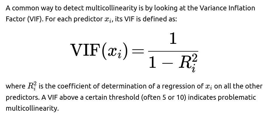
Variance Inflation Factor (VIF)

Practical Example (Python)

import numpy as np
import pandas as pd
from sklearn.linear_model import LinearRegression
from statsmodels.stats.outliers_influence import variance_inflation_factor

# Example dataset with correlated predictors
np.random.seed(42)
N = 100
x1 = np.random.rand(N)
x2 = x1 + np.random.normal(0, 0.1, N)  # correlated with x1
x3 = np.random.rand(N)

y = 3*x1 + 2*x2 + 1.5*x3 + np.random.normal(0, 0.1, N)

df = pd.DataFrame({'x1': x1, 'x2': x2, 'x3': x3, 'y': y})

# Fit a simple linear model
lr = LinearRegression()
lr.fit(df[['x1','x2','x3']], df['y'])
print("Coefficients (x1, x2, x3):", lr.coef_)

# Calculate VIF
X = df[['x1','x2','x3']]
vif_data = pd.DataFrame()
vif_data["feature"] = X.columns
vif_data["VIF"] = [variance_inflation_factor(X.values, i) for i in range(X.shape[1])]
print(vif_data)

Summary of Effect and Remedies

Correlated predictors can lead to:

• Inflated variances (standard errors) for the regression coefficients.

• Unreliable p-values and confidence intervals for the correlated terms.

• Difficulty in determining the true effect of each predictor on the response.

To address these issues:

• Use domain knowledge to remove or combine redundant features.

• Apply regularization (e.g., Ridge, Lasso) to penalize large coefficients and stabilize estimates.

• Perform dimensionality reduction (e.g., PCA) to transform correlated features into uncorrelated principal components.

• Monitor metrics like the Variance Inflation Factor to detect problematic multicollinearity.

By managing the correlation among predictors, you ensure your regression model not only predicts accurately but also yields more stable and interpretable estimates.

What if the correlated predictors do not inflate errors, but still affect model interpretability?

How does regularization help address multicollinearity?

Regularization methods add a penalty term to the cost function of ordinary least squares regression. This penalty term discourages large coefficient values when predictors contribute similar information. Specifically:

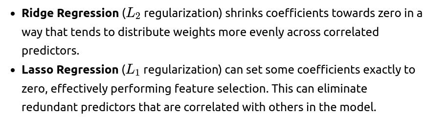
In Ridge Regression, the penalty term is:

where p is the number of predictors, and λ is a hyperparameter controlling the strength of regularization. This shrinks coefficients toward zero, distributing the weights more evenly among correlated predictors. Although it does not enforce exact zeros, ridge regression tends to reduce the magnitude of coefficients and helps stabilize them when features are correlated.

In Lasso Regression, the penalty term is:

Lasso performs both coefficient shrinking and can drive certain coefficients to zero, effectively removing some predictors from the model. When features are highly correlated, lasso tends to pick one (or a small set) of them and reduce or eliminate the others.

By doing so, regularization can mitigate some of the instability in coefficient estimates caused by correlated features, improving the interpretability and generalization of the model. However, you will need to tune the regularization hyperparameter (λ) via techniques like cross-validation to find a balance between bias and variance.

When might correlated predictors actually be beneficial?

Sometimes correlated predictors might be useful if your sole goal is predictive performance and each predictor captures subtle variations in the data. If removing any one of them degrades the predictive accuracy, you might prefer to keep them all, even if they are highly correlated. For example:

• In complex real-world datasets (like in image or text embeddings), certain features might indeed overlap in information, yet collectively contribute to better performance.

• Ensemble approaches or larger models (like deep neural networks) can sometimes handle correlated features without severe interpretability drawbacks if interpretability is less of a concern.

Nevertheless, if interpretability is important, correlated predictors can obscure which features are responsible for predictive power.

Could Principal Component Analysis (PCA) reduce interpretability?

Yes. PCA transforms the original features into new features (principal components) that are orthogonal to each other. This transformation often helps reduce the effects of multicollinearity. However, the new features are linear combinations of the original ones, which means they may no longer have straightforward physical or conceptual meaning.

In some settings, the first few principal components can have a clear interpretation, but often domain experts find it more difficult to relate principal components to real-world factors. As a result, while PCA is extremely useful for mitigating multicollinearity and improving model performance in some scenarios, you will be trading off a degree of interpretability.

How do you detect and confirm multicollinearity besides using VIF?

While VIF is a popular method, there are additional approaches:

• Correlation Matrix: You can compute the correlation matrix of your predictors and look for high absolute correlations (e.g., above 0.8). This is a quick way to spot pairs of correlated features.

• Eigenvalues of the Correlation Matrix: If the correlation matrix of predictors has one or more eigenvalues close to zero, it suggests a near-singular matrix, implying strong multicollinearity.

• Condition Number: The condition number of the design matrix can help detect potential numerical instability issues. A large condition number indicates possible multicollinearity.

In general, a combination of these approaches (e.g., correlation matrix plus VIF) provides a more comprehensive picture.

What if your model is purely predictive and you do not care about coefficient interpretability?

If interpretability is not a requirement and your main focus is on predictive accuracy, having correlated predictors is often less detrimental. Many modern machine learning methods, such as tree-based ensembles (Random Forest, Gradient Boosted Trees) or neural networks, can handle correlated features without significant issues for prediction tasks. Correlated predictors may still occasionally lead to overfitting, but typically cross-validation and careful hyperparameter tuning will handle that.

In such purely predictive settings, the presence of multicollinearity is less of a concern, although some methods (like linear models) still benefit from forms of regularization to avoid overfitting or unstable coefficients.

How do you decide which method to use for dealing with correlated predictors?

You might look at:

• Interpretability Requirements: If you need clear interpretability, removing or combining redundant predictors might be preferred to PCA. Lasso could help by zeroing out some coefficients, but keep in mind it can pick somewhat arbitrarily among correlated variables.

• Domain Knowledge: If domain knowledge indicates certain variables are proxies for the same concept, you can remove or combine them.

• Predictive Accuracy: If you mainly care about accuracy, you can keep them all and simply use a regularized model or a non-linear model, validating that you are not overfitting.

• Data Dimensionality: If you have a large number of features (e.g., text or image data), dimensionality reduction approaches like PCA can be essential for reducing computational complexity and mitigating overfitting.

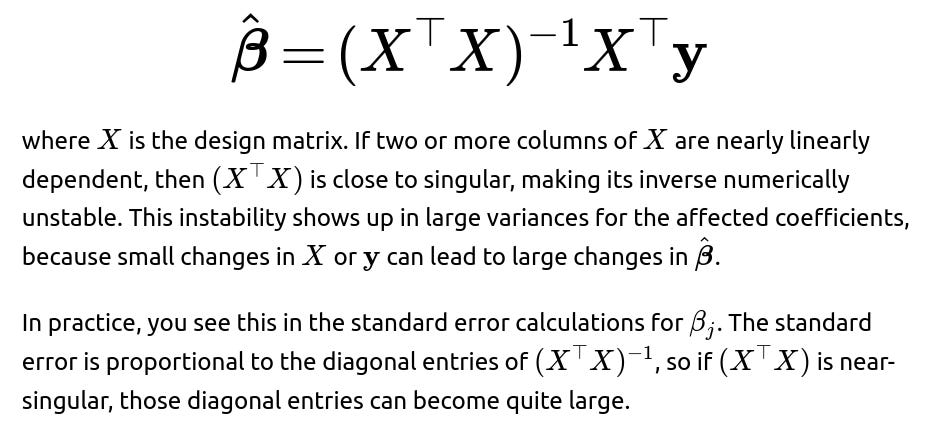
How would you formally explain why multicollinearity inflates variances of the coefficients?

Mathematically, in the Ordinary Least Squares estimate, the coefficients are typically solved by:

In summary

Correlated predictors in multiple linear regression can undermine coefficient estimation and interpretability. A model may still predict well, but the interpretability of the effects of individual predictors declines because small data changes can significantly alter their estimated coefficients. There are practical solutions—including using domain knowledge to reduce or merge predictors, applying regularization techniques (Ridge, Lasso), performing dimensionality reduction (PCA), or switching to other machine learning methods that handle correlated variables gracefully.

Each approach has trade-offs involving interpretability, ease of implementation, and predictive accuracy. Ultimately, the choice depends on your priorities (interpretation vs. prediction) and the specific characteristics of your data.

How to Answer Real Interview Follow-up Questions About This Topic

Explain the underlying linear algebra reasons for the inflation of variances and show that you understand how removing or combining correlated predictors can help. Demonstrate awareness of domain knowledge, regularization, and dimensionality reduction techniques. Provide examples in Python to illustrate how to detect and handle correlated predictors. Emphasize that whether multicollinearity is a problem can depend on whether your end goal is inference about individual predictors or purely predictive accuracy.

Below are additional potential follow-up questions with detailed answers:

Suppose you find a pair of highly correlated predictors. Should you automatically remove one?

It depends on your goals. If you are optimizing purely for predictive performance and not interpretability, you might leave them if they both contribute to a better model. Many modern algorithms (like random forests or gradient-boosting) are robust to correlated variables. However, for a linear model where interpretability is key, removing one may simplify the model and stabilize coefficient estimates. A pragmatic approach is:

• Check if removing one predictor degrades model performance (via cross-validation).

• Consider whether domain knowledge indicates they measure nearly the same property.

• Consider regularization to mitigate the effects of multicollinearity.

Does centering variables or standardizing them help with multicollinearity?

Centering or standardizing features does not eliminate the fundamental correlation among them, so it does not solve multicollinearity. However, it can improve the numerical stability of the design matrix and make it easier for regularization methods (like Ridge or Lasso) to converge. Standardization is also often recommended before applying PCA because PCA is sensitive to the scale of variables. While scaling helps from an optimization perspective, it will not remove the underlying correlation problem itself.

Is there any scenario where multicollinearity can cause the regression to fail to fit?

In more simpler terms, When we do a simple regression with one predictor, we can solve for the best-fitting line without much trouble because there is only one way to explain the variation in the outcome using that predictor. However, when multiple predictors are involved, we rely on a matrix (often called ( X^\top X )) to summarize how these predictors combine and influence the outcome.

For linear regression to find a unique best-fitting solution, that matrix must be invertible. Think of "inverting" a matrix as looking for a unique way to reverse its operation.

Imagine you have a simple arithmetic problem: you know that (3\times 4=12), so if someone only told you “the result is 12 and one factor is 3,” you could figure out that the other factor must be 4 (that’s the unique solution). In math terms, you can “invert” 3 (divide 12 by 3) to find 4.

Now picture a more complicated setup with multiple numbers all multiplied in some combination to give the final result. In linear regression, this is handled by a matrix equation. If the matrix can be “inverted,” you can uniquely solve for the regression coefficients, much like dividing 12 by 3 to get 4.

But how is invert 3 (divide 12 by 3) and a matrix inversion are the same concept?

They are the same concept, just in different dimensions. When you have a single number (a), multiplying something by (a) can be undone (or “inverted”) by dividing by (a). In matrix terms, you can think of (X) as a more complex version of that number (a). Instead of regular multiplication and division, you have matrix multiplication and matrix inversion. The idea is the same: if a matrix (X) is invertible, you can “undo” its multiplication by applying (X^{-1}). However, just as you cannot divide by zero in regular arithmetic, you cannot invert a matrix that has “zero-like” problems (such as when two columns are exact duplicates). That renders the matrix non-invertible, meaning there is no unique way to reverse what it does.

So when the matrix can’t be inverted—because some columns are just repeating each other’s information—there is no unique way to split up the effect among all those columns. It’s like being told the product is 12 but two of the factors are the same unknown number; there are multiple possibilities, so you can’t solve for a single unique value. That’s what makes regression fail in the case of perfect multicollinearity.

i.e. if one predictor is an exact linear copy of another—say one column is just double or triple another—then the matrix encodes the same information twice. Because there is no additional unique information, the matrix is said to be singular, which means it cannot be inverted (you can't reverse an operation that was essentially duplicated). In practical terms, there is no single best way to disentangle the effects of each predictor, so the algorithm does not know how to assign each predictor's contribution uniquely.

When this happens, the software might respond by throwing an error or automatically dropping one predictor from the perfectly collinear pair, ensuring that the matrix now has a unique solution. This avoids the "there’s no unique solution" problem and allows the regression to run properly.

Can stepwise regression help in dealing with correlated predictors?

Stepwise regression (e.g., forward selection, backward elimination) can sometimes remove correlated predictors. However, stepwise methods have known drawbacks, including potentially overfitting and failing to find the true best subset of predictors due to local optima in the selection process. They also ignore the effect of collinearity on the model’s interpretability. Hence, while you might see stepwise regression prune redundant predictors, more robust methods like regularization or domain-driven feature selection are often preferred.

Could partial least squares (PLS) be used to handle correlated predictors?

Yes. Partial Least Squares (PLS) is similar in spirit to PCA but specifically seeks to find latent components that both maximize variance in X and also have a strong relationship with the target y. This can often outperform PCA if the goal is predictive modeling, particularly when you suspect strong correlations among features. However, as with PCA, the latent components lose some direct interpretability in terms of original predictors.

Does using polynomial features or other feature engineering steps exacerbate correlation?

In practice, how do you typically approach this if you see correlated predictors in your data?

A practical workflow might be:

• First, measure correlation among predictors using a correlation matrix or VIF.

• If a pair of features is highly correlated, check domain knowledge to see if one is redundant.

• If you must keep both, try a regularized regression (ridge or lasso) to stabilize the coefficients.

• Evaluate model performance using cross-validation (both interpretability and predictive metrics).

• If interpretability is still problematic, consider PCA or partial least squares if appropriate, but keep in mind you lose a direct link to the original predictor space.

You should weigh these steps depending on your objective. For interpretability, you might favor removing redundant features or using lasso. For predictive performance, you might be more tolerant of correlated features if your chosen algorithm (like tree-based methods) handles them gracefully.

That concludes the in-depth discussion of how correlated predictors affect multiple linear regression and how to deal with them.

Below are additional follow-up questions

Is there a scenario where predictors might appear correlated due to small sample size or data anomalies?

If the dataset is small, random fluctuations can inflate correlation measures between predictors. For example, with very few observations (like 10–20 data points for a high-dimensional dataset), even purely random variables can show moderate to high correlations by chance. Data anomalies such as outliers can also artificially inflate or deflate correlations.

When you see a high correlation but suspect it might be due to limited data or outliers, you could:

• Collect more data: Increasing the sample size often provides a more reliable estimate of correlation.

• Perform robust correlation analysis: For instance, check Spearman’s rank correlation in addition to Pearson’s correlation, or use robust estimators less sensitive to outliers.

• Conduct sensitivity analysis: Remove outliers or run multiple experiments with different subsets of the data to see if correlations remain consistently high.

• Use domain knowledge: Sometimes the correlation is unexpected. Investigate whether a particular subgroup or data-collection artifact might be driving the relationship.

A potential pitfall is making a strong conclusion about collinearity based on an artifact. You might drop a feature or re-engineer your model unnecessarily, losing potentially valuable information if the correlation is spurious.

How do correlated categorical predictors differ from correlated numeric predictors in diagnosing and dealing with collinearity?

When dealing with categorical predictors (especially if they have many categories), correlation often manifests differently:

• For categorical variables, “correlation” is better expressed in terms of measures like Cramer’s V or the chi-square statistic. Two categorical variables might be associated if certain categories almost always co-occur.

• Dummy variables: When categorical features are encoded as one-hot vectors, certain dummy variables can become highly collinear. For instance, if one category is extremely common compared to others, the presence or absence of that category might mirror another category’s dummy variable distribution.

• Treatment of collinearity: Similar to numeric features, if dummy variables from different categorical encodings are highly correlated, standard multiple linear regression can still suffer from large coefficient variances. The remedy might be removing or merging categories, or using regularization methods.

A subtlety here is “perfect separation” in logistic regression (a related issue) where certain categories of a predictor perfectly predict the response. That can lead to infinite coefficient estimates, analogous to the perfect collinearity scenario in linear regression.

Practically:

• For many categories, consider merging infrequent categories to avoid overly sparse dummy variables.

• Check correlation or association metrics specifically designed for categorical features rather than just Pearson correlations.

• Use regularization (like Lasso or Ridge) when you have a large number of categorical features, which helps ensure stable estimates.

How does collinearity affect models beyond linear regression, such as logistic regression or generalized linear models?

Multicollinearity can also affect logistic regression or other generalized linear models (GLMs) in much the same way it affects linear regression. The fitting procedure for logistic regression maximizes the log-likelihood rather than minimizing squared errors, but the conceptual mechanics are similar: the design matrix can become close to singular if predictors are correlated, leading to:

• Large standard errors for the coefficients.

• Unstable parameter estimates that can vary significantly with small changes in the data.

• Potential misinterpretation of which variables meaningfully affect the odds of the outcome.

In extreme cases, if one predictor is nearly a linear combination of others in logistic regression, the optimization may fail to converge or produce very large coefficient magnitudes.

To handle this:

• Use Ridge or Lasso regularization in logistic regression (commonly called “logistic regression with a penalty term”). This helps stabilize coefficient estimates in the presence of correlated features.

• As with linear regression, check a variant of the Variance Inflation Factor (adapted for logistic regression) or examine correlation matrices to identify highly correlated predictors.

• Consider removing or combining redundant predictors if interpretability is crucial, or rely on regularization if prediction is the key objective.

Can domain knowledge be used to create synthetic or derived features that reduce correlation?

This approach can:

• Reduce dimensionality if multiple correlated variables are combined into a smaller set of uncorrelated or less-correlated features.

• Improve interpretability if the derived feature has a clear, domain-driven interpretation (e.g., “temperature fluctuation range”).

• Avoid dropping variables blindly by using domain understanding to keep meaningful contributions from each original variable.

The edge case here is when you combine features incorrectly or in a way that adds noise. Always test with cross-validation to see if the combined feature genuinely helps performance or interpretability compared to the original features separately.

How might outliers or non-linear relationships exacerbate or mask correlation among features?

Outliers can drastically affect the Pearson correlation coefficient. A single extreme point can either inflate or deflate the observed correlation, making two features appear correlated (or uncorrelated) when, in fact, the majority of data does not reflect that relationship. Similarly, non-linear relationships—like a curved relationship between two features—might go unnoticed if you only measure linear correlation.

In practice:

• Use robust methods or transform the data to reduce the impact of outliers. For instance, applying log or rank transformations might lessen the skew and mitigate outliers’ influence.

• Examine scatter plots to see if the relationship between two features is non-linear. A high “linear” correlation might just be one part of a more complex association.

• If non-linearity is suspected, consider polynomial or spline transformations carefully. But note that adding polynomial features can further increase collinearity if not managed properly.

• Use correlation measures (like Spearman’s rank correlation) that can capture monotonic relationships, or more sophisticated methods (like mutual information) that can detect broader patterns.

Is it possible that correlated features lead to incorrect causal inferences or confounding?

Yes, correlated predictors can obscure true causal relationships. If you rely on multiple linear regression for causal inference rather than mere correlation, you typically assume no unmeasured confounders and that the included variables are not perfectly collinear. However:

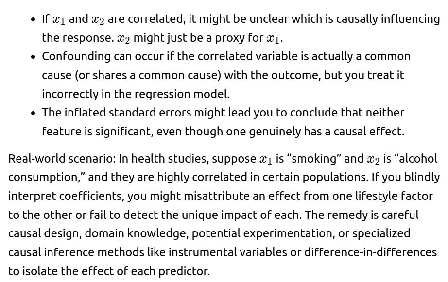
How might advanced neural network architectures handle correlated features differently than linear models?

Neural networks—especially deep architectures—have internal layers that can learn transformations of the input space. In principle, a neural network can discover a suitable representation that mitigates redundancy among correlated features. For instance, early layers might combine correlated inputs into more independent representations.

However, correlation can still affect:

• Optimization: If two inputs convey nearly identical information, the network might require more epochs or specialized initialization to converge to a stable set of weights.

• Overfitting: Redundant inputs could increase the chance of overfitting unless there is regularization (e.g., dropout, weight decay, or batch normalization).

• Interpretation: With a highly flexible model like a deep neural network, correlated inputs add to the complexity, making it even harder to interpret which features matter.

In many practical cases, data preprocessing techniques—like dimensionality reduction or domain-driven feature selection—still benefit neural networks by reducing input redundancy, potentially leading to faster training and better generalization.

Could correlation among features hamper gradient-based optimization in deep learning?

Yes, strong correlation among features can lead to poor conditioning of the weight space. In gradient-based optimization, especially if batch sizes are small or if the correlation structure is complex, you can observe:

• Slow convergence: The network has to “unravel” redundant patterns in early layers, which might take many gradient updates.

• Sensitivity to initialization: Highly correlated inputs might cause certain neurons to learn overlapping patterns, leading to local optima or plateaus if initialization isn’t well-tuned.

• Need for normalization: Techniques like batch normalization can partially address the issue by normalizing intermediate feature distributions, thereby easing optimization in the presence of correlated activations.

Although deep neural networks are often robust to mild to moderate input correlation, extreme cases of redundancy can still pose challenges. Testing with or without correlated features, or applying dimensionality reduction before training, can show whether correlated features slow training or degrade performance.

Could correlated predictors cause issues during cross-validation or model selection?

In cross-validation, you partition the data into folds and train/test multiple times. If your features are highly correlated, certain folds might contain slightly different distributions of those correlated features. Potential pitfalls:

• Variance in coefficients: The model might learn drastically different coefficient estimates across folds, making model selection or hyperparameter tuning difficult.

• Overestimation of performance: In some cases, correlated features might lead your model to latch onto spurious patterns that happen to be consistent across folds. If the correlation is accidental, the cross-validation estimate might be overly optimistic.

• Feature selection confusion: If you use methods like stepwise selection or Lasso for feature selection within each fold, different correlated predictors might be chosen, leading to an inconsistent set of “best” features across folds.

A best practice is to ensure that any feature engineering or selection steps are done inside the cross-validation loop to avoid data leakage. Also, if correlation is severe, you might see unstable performance estimates from fold to fold, indicating you should either remove or merge redundant variables or apply a robust regularization method.

What if I have partial correlation among multiple sets of variables and want to isolate each group’s contribution?

Partial correlation measures the relationship between two variables while controlling for the influence of others. In regression contexts, if you have multiple clusters of correlated predictors, you can examine partial correlations within each cluster, conditioning on the rest of the features.

However, partial correlation might still be tricky to interpret if your variables overlap in multiple ways. Additional approaches include:

• Hierarchical regression: Enter groups of correlated variables in stages, observing how the model’s explained variance changes. This can help you see which cluster of variables contributes incremental explanatory power.

• Multilevel modeling: If the correlation structure is due to hierarchical data (e.g., individuals nested within groups), a multilevel model can partition variance at different levels.

• Canonical correlation analysis: If you have two sets of variables (e.g., group A and group B), canonical correlation can find linear combinations within each set that are maximally correlated. This may help you understand how entire blocks of features relate to each other and to the response, though it’s more of an exploratory tool than a straightforward fix to multicollinearity.

Pitfalls here include over-complicating the model and losing interpretability. Always weigh the benefit of precisely dissecting correlated groups against the added complexity in your final model.

What are some edge cases where dimensionality reduction (e.g., PCA) could fail to improve the model?

Dimensionality reduction techniques like PCA assume that the directions of maximum variance in the feature space also contain the most useful information for the predictive task. However:

• If the target variable is associated with a direction of low variance in your predictor space, PCA might discard or down-weigh that direction. The principal components capturing the largest variance might not correlate strongly with the outcome.

• If your features are non-linearly related, linear PCA might not capture the true structure. Kernel PCA or other non-linear methods might be needed, but these can be more complex and less interpretable.

• If your dataset is extremely small, the PCA transformations might be unreliable or too sensitive to outliers, introducing more noise than clarity.

In these scenarios, you could test partial least squares (PLS), which tries to find latent components that maximize covariance with the target, or attempt domain-informed transformations that specifically aim to preserve the relationship with the response variable.

Could correlated predictors ever be used to intentionally obscure interpretability?

Yes, though this is more of an organizational or ethical concern than a technical one. If multiple correlated variables are introduced, the coefficients of any single one might become unclear. In some contexts—like model obfuscation—individual feature importances can be hard to discern. While it’s not typically a best practice in most data science work, in certain competitive or proprietary environments, correlated features could make it difficult for external observers to replicate or interpret the model.

From a purely technical perspective, this scenario demonstrates that while correlated features do not necessarily harm predictive power, they do obscure the clarity of how each feature influences the outcome.

How can ensemble methods, like random forests, handle correlated predictors?

Tree-based methods, including random forests and gradient-boosted trees, often handle correlated predictors with greater ease because:

• Individual trees pick split points among available features, and random forest algorithms typically sample subsets of features at each split, reducing the dominance of any one correlated feature.

• Even if two or more features are correlated, they can still appear in different branches of different trees. The ensemble then averages or aggregates these splits.

However, pitfalls include:

• If one correlated predictor is slightly more predictive, it might dominate splits, causing other correlated features to be used less frequently, leading to potential biases in variable importance measures.

• If you rely on feature importance metrics such as Gini importance, correlated variables might share credit in an unpredictable manner or appear artificially less important. Permutation-based importance can also be distorted if features are correlated.

You can still benefit from dimension reduction or removal of highly redundant variables to simplify the model, reduce training time, and potentially improve interpretability. But from a purely predictive standpoint, random forests often remain quite robust to moderate levels of correlation among features.

How does multicollinearity impact confidence intervals and hypothesis testing in frequentist statistics?

• Confidence intervals: They widen, reflecting greater uncertainty about the coefficient estimates.

• t-tests or F-tests for coefficients: p-values can become large (loss of statistical significance), even if one of the correlated predictors is truly influential.

• Overall model tests (e.g., the F-test for overall significance): They may still indicate the model is significant, but you cannot parse out the significance of individual predictors well.

A subtle edge case: Two or more correlated predictors can “share” explanatory power to the point that each looks non-significant individually, yet removing them collectively harms the model. This discrepancy can confuse interpretation if you only rely on individual p-values without looking at the full model fit or partial F-tests that consider groups of predictors together.

If correlation among predictors changes across time, how do you handle that in a time-series setting?

Time-series data often exhibits correlation patterns that shift over different periods. For instance, two economic indicators might be correlated during a recession but less correlated during a boom. Dealing with time-varying correlation can involve:

• Splitting data into different time intervals and fitting separate models or including interaction terms with a time component to capture evolving relationships.

• Rolling-window analysis or rolling correlation: Periodically estimate correlation in a sliding window to see how it changes. This can inform whether you treat certain predictors as near-collinear in all periods or only in specific intervals.

• Regularized dynamic models: Techniques like state-space models with shrinkage or time-varying parameters can adapt coefficients over time, potentially mitigating issues from correlation that only appears in some intervals.

An edge case is if you incorrectly assume constant correlation across all time, leading to an over- or underestimation of coefficient variances. Always investigate whether the correlation is stable throughout the entire time series before deciding how to treat collinearity.

Are there Bayesian approaches to deal with correlated predictors?

Yes. In a Bayesian regression framework, you place prior distributions on coefficients. If you suspect collinearity, you can use informative or partially informative priors that shrink coefficients toward zero or toward each other if you know they measure similar phenomena. Examples:

• Hierarchical priors: Group correlated predictors under a common hyperparameter, effectively sharing statistical strength and reducing the risk of large, unstable estimates for any single predictor in the group.

• Bayesian ridge and lasso: The Bayesian analogs of frequentist Ridge and Lasso can stabilize coefficients through the prior structure.

Pitfalls:

• Specifying priors requires careful thought. Overly strong priors might bias coefficients too much toward zero or incorrectly assume a certain form of correlation.

• If you have minimal domain knowledge, purely data-driven priors might not fully solve collinearity. But they can still perform better than an unregularized approach by preventing coefficients from blowing up.

Bayesian approaches often yield posterior distributions that reveal how uncertain each coefficient is. With correlated predictors, you might see wide posterior intervals that reflect the difficulty in distinguishing their individual effects. This transparent uncertainty can be an advantage in interpretation compared to frequentist point estimates that might flip signs or vary widely with small data changes.

Could a high correlation among predictors ever be exploited to detect data leakage?

Yes. Sometimes, suspiciously high correlation between certain features can signal unintended data leakage. For instance, if a feature is effectively a disguised or leaked version of the target, you might spot an unusually strong correlation with other relevant predictors or with the target variable itself. This can happen when:

• A process that generates your training data inadvertently includes future information or post-outcome data.

• A proxy variable is capturing nearly the same information as the target or is updated after the target is determined.

When you detect extremely high correlation, especially near 1.0 or -1.0, investigate whether that feature is legitimately measuring something in real-time or if it’s a data leakage artifact. If it’s leakage, you must remove or re-engineer that feature to preserve the integrity of your model.

Could correlated predictors impact partial dependence plots or feature attribution methods such as SHAP?

Yes, feature attribution methods like SHAP (SHapley Additive exPlanations) assume features contribute independently to the model output in a combinatorial sense. However, when features are correlated, the attributions can become more complex:

• In the presence of correlation, if two features explain mostly the same variance, the model might arbitrarily assign credit to one feature in some instances and the other feature in others. This can yield attributions that seem inconsistent with domain knowledge.

• For partial dependence plots (PDPs), if you vary one feature while holding others constant, it might be an unrealistic scenario in real data. Highly correlated features typically move together, so a PDP that changes one while keeping the correlated feature fixed might not reflect typical real-world relationships.

In practice, you can:

• Use conditional PDPs or variable dependence plots that account for the average relationship between correlated features.

• Interpret SHAP values with caution in correlated feature settings, possibly grouping correlated features or using hierarchical attributions to see joint effects.

• Cross-check with domain knowledge to confirm that the attribution method is not attributing an effect to the “wrong” correlated variable due to how the Shapley values distribute credit.

Such pitfalls highlight that interpretability techniques also need to account for multicollinearity in the data to provide faithful explanations.

How should you document and communicate findings about correlated predictors to stakeholders?

Clear communication about correlations and their implications is crucial. Many stakeholders—like product managers or executives—might expect a single “best” feature to explain outcomes. In the presence of correlated predictors, you should:

• Show correlation matrices or simpler visualizations (like pairwise scatterplots) to illustrate redundancy.

• Explain how correlated predictors inflate standard errors and hamper the interpretability of individual coefficients.

• Present whether you used techniques like PCA or Lasso to reduce redundancy and why.

• Emphasize that the overall model might still be valid for prediction but that attributing the outcome to one specific predictor might be misleading.

Pitfalls:

• Over-technical explanations: Some stakeholders might be overwhelmed by VIF, partial correlation, or advanced methods. Translate these into accessible language without losing critical nuance.

• Under-communication: Failing to mention that your model includes many correlated features could lead to misguided decisions, especially if stakeholders think each predictor is independently driving the outcome.

Effective documentation includes which steps were taken (feature removal, regularization, dimensionality reduction, etc.), the rationale behind them, and how each decision impacted both predictive performance and interpretability.

Could correlation among predictors be desirable if you need to model interactions?

• Consider regularizing the entire model or specifically the interaction term to avoid large coefficient swings.

• Use domain insights to limit the interaction terms only to those pairs of variables where a meaningful interaction is hypothesized.

• Check cross-validation performance to ensure interactions are truly beneficial rather than overfitting.

Even if correlated features can hint at interesting interactions, the same correlation can undermine stable estimation unless carefully controlled with methods like regularization or hierarchical modeling.

Could correlation among predictors be a sign that we need a different modeling approach altogether?

Yes. In some cases, having many strongly correlated features might reveal an underlying latent structure in your data that a linear model is not capturing efficiently. Alternative approaches might include:

• Factor analysis or latent variable models: If multiple observed features are all related to a smaller set of unobserved latent variables.

• Non-linear machine learning models: Tree-based or neural network models might be more flexible in capturing complex patterns among correlated features.

• Graphical models or structural equation models: If you believe there is a network of dependencies between predictors and outcomes, you might want to explicitly encode those relationships.

A pitfall is blindly forcing a multiple linear regression or logistic regression framework when the data structure suggests a fundamentally different approach. Identifying correlation can be the first clue that your data is more complex than your initial modeling strategy assumed.

In what way does collinearity relate to the concept of the rank of the design matrix?

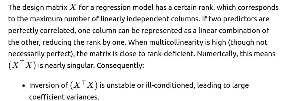
• Small numerical errors in the data or rounding during computations can produce disproportionately large fluctuations in estimates.

Edge case: If the rank is actually lower than the number of predictors due to perfect multicollinearity, many software packages will automatically drop or combine redundant columns. However, near-perfect collinearity often remains undetected unless you explicitly check VIFs or condition numbers, so you could inadvertently have a rank-deficient or near-rank-deficient problem.

How might correlated predictors affect online or incremental learning?

In online learning, the model updates its parameters as new data arrives in a streaming fashion. If two or more features are highly correlated:

• The gradient updates might become unstable or oscillatory if the learning rate is not carefully tuned, especially in algorithms like stochastic gradient descent (SGD) where you update parameters incrementally.

• With correlated features, the model might overemphasize whichever feature’s gradient it happens to see first, leading to suboptimal parameter convergence or slow adaptation.

• Over time, if correlation changes in new incoming data (e.g., concept drift), the previously learned model parameters might no longer be valid. You’d need to adapt or re-train the model more aggressively.

Practical tips include ensuring a well-conditioned design through dimension reduction or regularization from the outset. Continually monitoring feature correlations in a streaming context can alert you to distribution shifts that demand re-calibration or more advanced online regularization methods.

Does collinearity ever change how we approach missing data imputation?

When imputing missing data, especially if you use regression-based or model-based imputation methods, correlated variables can provide valuable information to fill in the missing values. However:

• If variables are collinear, your imputation model may become unstable or yield imputed values that mirror the redundancy.

• Perfect or near-perfect correlation can lead the imputation algorithm to produce duplicate or deterministic values for the missing entries, reducing variation in the dataset.

• Multiple imputation procedures can also reflect the increased uncertainty in collinear settings, resulting in broader confidence bounds when combining imputed datasets.

  

  What are some practical ways to confirm that removing one of a pair of correlated features is beneficial?

  After you spot a pair of correlated features, you can test dropping one:

  1. Cross-Validation Performance: Train the model with all features versus a model with one of the correlated features removed. If performance remains the same or improves, dropping that feature is likely beneficial.

  2. Coefficient Stability: Observe how coefficients change across folds. If removing the feature stabilizes the estimates and does not degrade accuracy, it’s an indication that the removed feature was redundant.

  3. Model Complexity: Fewer features can lead to simpler, more interpretable models. If you see no significant drop in performance, parsimony is often preferable.

  4. Domain Suitability: Check domain expertise. Perhaps the dropped feature was less reliable or more expensive to measure in a production environment.

  Pitfalls:

  • Overly simplistic approach: You might remove a feature that has subtle but critical contributions in certain subgroups of the data.

  • Short-sighted evaluation: If your test set is not large or representative, you might incorrectly conclude that removing a feature has no impact. Always do robust testing with an appropriate dataset size.

  If a model with correlated predictors is used in production, can the correlation shift over time and what are the implications?

  Yes. Correlations in real-world data can change over time (concept drift). For instance, two consumer behavior metrics might be closely correlated during certain economic conditions but diverge later. If your production model assumed their stable correlation, you might experience:

  • Degradation in predictive performance: The model’s learned coefficients, reliant on historical correlation structure, no longer generalize.

  • Interpretation errors: If you interpret the model coefficients in a changed correlation regime, you might incorrectly attribute changes in the outcome to one predictor when it’s really due to the drift in how features relate to each other.

  Continuous monitoring of feature statistics—including correlation matrices—can alert you to distribution shifts or changes in correlation. You may need to retrain or update your model periodically, possibly implementing an online or incremental learning approach that adapts as correlations change. This is especially relevant in dynamic industries like finance, e-commerce, or social media trends where user behavior patterns evolve rapidly.

  Does strong correlation among features ever hint that the data gathering process should be revised?

  Often, yes. For instance, if two sensors in an industrial process measure nearly identical signals, the correlation might approach 1.0. This duplication might indicate wasted resources collecting redundant data. Alternatively, it might be intentional for validation or failover in case one sensor fails. Understanding the reason behind correlation can inform:

  • Future data collection: You might reduce cost by eliminating or redesigning redundant data sources.

  • Data quality checks: If two sensors are expected to measure different phenomena but yield nearly identical readings, there could be a malfunction or calibration issue in one sensor.

  • More efficient data integration: If multiple channels gather overlapping information, you might unify them into a single reliable measure rather than storing multiple streams.

  Edge cases here revolve around ensuring you do not remove redundancy that is operationally or quality-assurance critical. Redundant sensors or measurements are sometimes necessary for fault tolerance, so a high correlation might be intentional rather than a problem to fix.

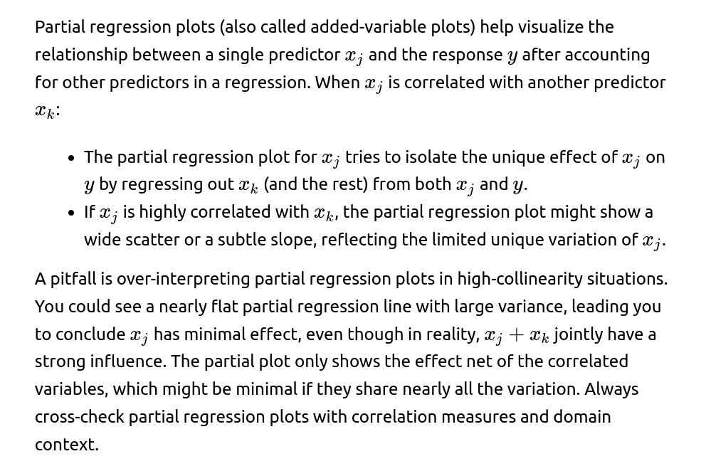
  Does collinearity affect how we interpret partial regression plots?

  

  How do you adapt cross-feature constraints when dealing with correlated variables?

  

  What if the correlation structure is non-stationary in a spatial context?

  Spatial data often exhibits location-based correlation among features (e.g., geographic variables or local measurements). Non-stationarity means the correlation structure can vary by region. This can pose challenges:

  • Global regression models might incorrectly assume the same level of correlation everywhere, leading to poor fit in certain regions.

  • Geographically Weighted Regression (GWR) or spatially varying coefficient models can adapt to local correlation structures. However, diagnosing multicollinearity becomes more complex because each location or region might have a different correlation pattern.

  • If two spatial variables are correlated in one area but not in another, a single global coefficient can become misleading.

  You might split your data by region, fit separate models, or use a hierarchical or spatially-aware modeling technique that accounts for local correlation differences. The pitfall is ignoring spatial heterogeneity, which can mask or inflate correlations when you aggregate data across large geographic areas.

  Could correlated predictors still be useful for generating counterfactual explanations?

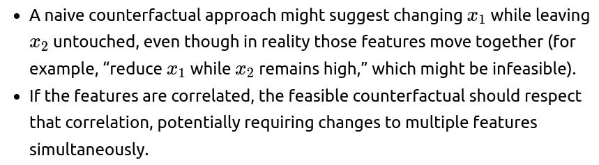
  Counterfactual explanations typically attempt to find minimal changes to input features that alter the predicted outcome. In the presence of correlated features:

  

  Advanced counterfactual methods can incorporate correlation constraints or use generative models that ensure proposed counterfactual instances are realistic. A pitfall is generating counterfactuals that are not actionable or realistic because they violate the actual correlation structure observed in the real world. A robust solution ensures that any changes to one feature also reflect expected changes in correlated features.

  If a deep model is used and we do not explicitly remove correlated features, do we still need to worry about it?

  While deep neural networks can sometimes “learn around” correlated features, there are still practical reasons to worry:

  • Training time and resources: Redundant features can lengthen training or require more parameters, leading to higher computational cost.

  • Overfitting: Even with regularization, a surplus of correlated features can encourage the network to memorize spurious patterns.

  • Interpretability: Although deep networks aren’t always used for interpretability, correlated inputs can further obscure the partial contributions of each feature.

  • Data shift resilience: If correlation among inputs changes in real-world deployment, the model might not generalize well unless it has learned an appropriate representation or you have enough data augmentation reflecting these shifts.

  So even though deep learning can handle correlation better than classic linear regression, ignoring it completely can create hidden vulnerabilities. A thorough data preprocessing pipeline (including feature selection, transformation, or dimensionality reduction) can yield more robust neural network models in many cases.

  Could correlation indicate that a predictor is a transformation of another variable (e.g., scaled, log-transformed, etc.)?

  

  In these cases, decide if you need both versions. Often, one form might be more linear in relation to the outcome, leading to a simpler model with fewer non-linearities. Alternatively, you might keep the log-transformed version if it better satisfies normality assumptions. The pitfall is including both in the same regression, which rarely adds interpretive value and can inflate variance estimates unnecessarily.

  Always check transformations so you do not inadvertently keep two nearly identical versions of the same data. Removing the redundant version typically simplifies the model and helps with interpretability.

  Does high correlation among features always imply that the model’s effective dimensionality is low?

  High correlation does imply redundancy, but not necessarily a low effective dimensionality in all cases. You could have multiple independent clusters of correlated variables, so your data might have a “block” correlation structure. Within each block, features are highly correlated, but across blocks, they’re independent. That means:

  • Locally, each cluster might only represent one or two underlying latent factors, reducing dimensionality within the block.

  • Globally, you might still have multiple blocks that each carries unique information, so the overall effective dimensionality is the sum across blocks.

  Pitfalls:

  • Overapplying a single-dimensionality argument when correlation is blockwise or structured. Each cluster might need separate dimensionality reduction or domain-based feature consolidation.

  • Failing to see that certain features across blocks could also have minor cross-correlations that become important in large-scale interactions.

  Hence, always look at the bigger picture of how your correlation matrix is structured, rather than focusing on pairwise correlations alone. A more holistic approach (like cluster analysis on the correlation matrix or advanced factor analysis) can help unravel the true dimensional structure.

  Are there specialized regression techniques designed specifically for correlated predictors besides Ridge/Lasso?

  Yes. Apart from the common regularization methods, there are more specialized approaches:

  

  Bayesian Group Lasso or Grouped Regularization: If you know in advance that certain features form a correlated group (say, all polynomial terms of a single variable), group lasso or hierarchical priors can be used to shrink entire sets of coefficients collectively.

• Sparse Partial Least Squares: Extends partial least squares but adds a sparsity constraint, helpful when the number of predictors is large and includes correlated blocks.

• Orthogonal Matching Pursuit: A greedy algorithm that picks features most correlated with the residual but can be adapted to skip or combine correlated features at each step.

Pitfalls with specialized methods include the need for careful hyperparameter tuning and domain knowledge to group features effectively. Without proper tuning or grouping, these methods could produce suboptimal or overly complex solutions.

What are real-world domains where collinearity is especially pervasive?

• Economics and Finance: Macroeconomic indicators (e.g., unemployment rate, inflation, interest rates) often move together, creating collinearity.

• Genomics: Gene expression levels can be highly correlated across certain biological pathways.

• Sensor Data/IoT: Multiple sensors measuring related physical phenomena can produce nearly duplicated signals.

• Marketing Analytics: Different channels (TV ads, online ads, social media presence) might correlate strongly because they scale together in large campaigns.

• Healthcare: Vital signs (heart rate, blood pressure, oxygen saturation) can rise or fall together under certain conditions.

The common thread is that correlated features often indicate underlying phenomena that couple the variables. The domain solution might be to identify and model those phenomena directly or use methods that handle collinearity gracefully.

When is it acceptable to ignore collinearity?

It can be acceptable to ignore collinearity in a few scenarios:

• Purely Predictive Tasks with Robust Models: If you are using methods like random forests, gradient boosting, or deep neural networks and do not require interpretable coefficients, correlation may not harm accuracy. You still might keep them for the model to discover any small but unique signals.

• Short-term Prototyping: If you’re quickly prototyping a model to see if any immediate signal exists, you might temporarily skip a detailed correlation analysis, especially if you plan to refine the model later.

• Very Large Datasets: With abundant data and stable parameter estimation (particularly if you’re employing regularization), mild to moderate correlation might not be a pressing issue.

A potential danger is that ignoring high collinearity can mask interpretability issues or lead to unpredictable shifts in coefficient estimates over time. Even in purely predictive tasks, if correlation changes unexpectedly in production data, ignoring it might lead to degraded performance. So “acceptable” is still context-dependent, and you should remain cautious if correlations are extremely high.

Does software automatically warn about multicollinearity, or do we need to check manually?

Most regression libraries (in R, Python, or other languages) do not automatically warn you about collinearity, unless it’s perfect (rank deficiency). In that perfect scenario, software may produce an error or automatically drop one column. But for high correlation that is not perfect, you typically have to check:

• Variance Inflation Factor (VIF) or condition number manually.

• Correlation heatmap or correlation matrix of predictors.

• Coefficient stability across repeated runs or cross-validation folds.

Pitfalls:

• Overreliance on default outputs: You might get a seemingly valid set of coefficient estimates with large standard errors, but no direct warning.

• In bigger models (like deep neural networks), libraries rarely comment on correlated inputs. Monitoring performance metrics or the stability of the training process is still on you.

Thus, diagnosing collinearity remains the responsibility of the data scientist or statistician. A thorough data exploration step that includes correlation checks is essential in best practices.

Are there special diagnostic plots or advanced visuals for exploring collinearity?

Beyond the standard correlation matrix or heatmap, you can use:

• Pairs Plot: A grid of scatterplots for every pair of features, giving an immediate sense of how strongly they correlate.

• Principal Component Biplot: Shows how each original feature loads on the principal components. If many features lie close together, it suggests high correlation among them.

• VIF vs. Feature Plot: A bar plot with VIF on the y-axis and features on the x-axis, highlighting which features have the largest inflation factor.

• Partial Correlation Network Graph: Displays nodes as features, edges weighted by partial correlation strength, giving a quick read on which subsets of variables are strongly intertwined.

Pitfalls include clutter in high dimensions—some advanced plots become difficult to interpret with dozens or hundreds of features. For large dimensions, focusing on subset-based or hierarchical approaches is often more tractable.

Could collinearity distort the interpretability of coefficients in polynomial or interaction expansions specifically?

• Difficulty interpreting the significance of higher-order terms if they are overshadowed by collinearity with the lower-order terms.

Hence, if you expect non-linearities, you might add polynomial features but also rely heavily on regularization to keep coefficients stable. Another approach is to use orthogonal polynomial expansions, which are constructed to be uncorrelated with each other, mitigating collinearity.

How do interaction terms with categorical variables further complicate collinearity?

When a categorical variable is expanded into dummy variables, and you create interactions with a numeric feature, each dummy variable can interact with that numeric predictor, leading to multiple new features. If the categorical has many levels (say 10 levels), that’s 10 new interaction terms with the numeric variable, potentially introducing correlation among the dummies and the numeric feature:

• Dummies can be correlated if one category is very frequent, overshadowing the others. The interaction terms with the numeric predictor might also share that frequency pattern, compounding correlation.

• The numeric predictor itself might strongly correlate with its own interaction terms if not properly centered or scaled.

Therefore, it’s prudent to carefully examine whether each interaction is warranted. Also, using domain-specific hypotheses to restrict which categories should interact with which numeric features can reduce correlation blow-up and keep the model interpretable.

If two features are correlated but have opposite signs for their regression coefficients, is that necessarily contradictory?

Not necessarily. Correlation simply indicates a linear relationship between two features, while the coefficients in a multiple regression reflect each feature’s partial effect controlling for the other.

For example:

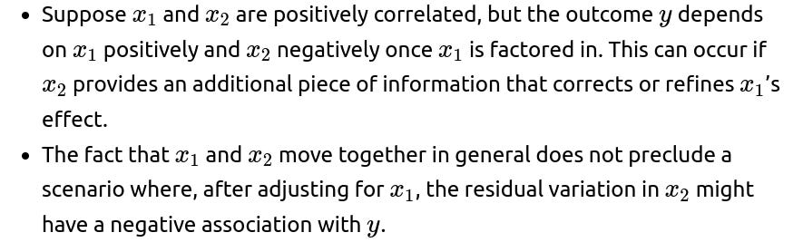
The pitfall is interpreting partial coefficients without acknowledging correlation. It might look strange at first that correlated features have coefficients with differing signs, but it can be a legitimate outcome in a multiple regression model if they convey overlapping yet directionally distinct signals about y. Always cross-check with partial regression plots, domain knowledge, or tests for significance to ensure the negative sign is consistent with data patterns and not a spurious result of extreme collinearity.

How do you handle correlated features in Bayesian hierarchical models where each predictor belongs to a group?

In hierarchical models, you can introduce group-level effects or random effects. If you have correlated features within a group (e.g., multiple tests measuring cognitive ability in the same group of participants), you can:

• Specify a group-level prior that pools information across correlated predictors in the same group, shrinking them together. This may reduce collinearity’s impact by borrowing strength across group members.

• Add correlation structures at the group level: If you anticipate certain random effects are correlated, you can model their covariance matrix explicitly. This lets you capture the correlation in a structured way rather than ignoring it.

• Use partial pooling to reduce overfitting for each predictor. If two predictors are correlated, partial pooling can keep each one’s coefficient from becoming unduly large.

One pitfall is that specifying priors and correlation structures incorrectly can create misestimation. Overly rigid priors might flatten real differences, while under-specified correlation structures might let collinearity cause wide intervals. Careful model checking using posterior predictive checks or WAIC/LOO cross-validation can guide you to an appropriate hierarchical structure that handles correlated predictors gracefully.

How does a structural equation modeling (SEM) approach differ from standard regression in handling correlated predictors?

SEM allows you to specify latent variables, direct and indirect paths, and error terms for both observed and latent constructs. In SEM:

• Correlation among predictors can be modeled explicitly as correlations among latent factors or residual correlations among observed variables. You can separate measurement error from the constructs the variables are intended to represent.

• By imposing a theoretical causal structure, you can test specific hypotheses about how correlated predictors relate to each other and to the outcome.

• SEM uses fit indices (like RMSEA, CFI, TLI) rather than just R-squared or standard errors, so you can see how well your entire model (including correlated paths) fits the data.

Edge cases:

• Overfitting with a large number of parameters in complex models, especially if the data set is not large enough.

• Misspecification: If you incorrectly specify which variables are allowed to correlate, the resulting model can be biased or misfit.

• Identifiability: If the SEM includes many correlated paths, you might have identifiability issues analogous to rank deficiency in standard regression.

Thus, SEM can incorporate correlations among predictors more flexibly, but it demands rigorous theoretical justification and careful parameterization to avoid simply shifting the multicollinearity issue into a more complex model.

Could “too many” correlated features cause memory or computational issues?

Yes. While the main effect of collinearity is on coefficient estimation, a high-dimensional matrix X with many correlated columns can also become large, leading to computational difficulties:

• Storing large intermediate arrays for gradient-based methods becomes memory-intensive, particularly if you do repeated cross-validation or hyperparameter tuning.

Techniques like PCA, factor analysis, or random projection reduce dimensionality, diminishing both memory usage and computational cost. Alternatively, specialized solvers for large-scale linear systems can handle partial updates or streaming data. If you ignore the correlation and keep all features, you might run into practical scaling limits, especially in industrial or big-data contexts.

Could correlation indicate a data duplication or data entry error?

Absolutely. A surprisingly high correlation might mean that the same feature was recorded under two different names or loaded twice into the dataset by mistake. Sometimes data pipelines can inadvertently merge or replicate columns. This is especially likely if the features have identical or near-identical values for every sample.

Always do a quick sanity check for columns that are 100% identical or differ by a constant factor. Correcting data errors not only resolves collinearity but prevents modeling mistakes. A real-world example: A CSV file might contain “Age” and “Customer Age” columns that are identical or a second unintentional column with the same values. Recognizing this redundancy clarifies the feature space and avoids confusion in analysis.

How would robust regressions (like Huber or RANSAC) handle correlated predictors?

Robust regression methods mainly focus on reducing the influence of outliers in the response or in the predictors. High correlation among predictors still leads to:

• Instability in coefficient estimates for correlated features, though robust methods might mitigate extreme swings caused by outliers if those outliers affect some features more than others.

• If collinearity is severe, even robust methods can yield large variance or standard errors for the coefficients. They address outliers, not near-singularities in the design matrix.

Therefore, robust regression can handle unusual data points better, but it’s not a silver bullet for correlation issues. If correlation is the primary concern (rather than outliers), you still need to consider dimension reduction, regularization, or feature engineering.

If I see that two features are strongly correlated in all known datasets, can I safely assume they’ll remain correlated in future unseen data?

Not necessarily. Correlations can be domain-dependent and time-dependent. For example, in technology product analytics, user behaviors that correlate strongly during a product launch might diverge once the product matures. If you rely on that correlation for your model’s stability, you risk performance drops if future data deviates from historical patterns.

When building a model that depends on correlated features, it’s wise to:

• Validate across multiple datasets or time periods to ensure correlation remains relatively stable.

• Consider “stress-testing” your model with synthetic or scenario-based data to see how it behaves if the correlation decreases or reverses.

• Monitor correlation metrics in production, triggering alerts or re-training if correlation shifts significantly.

Failing to do so can lead to overly optimistic performance estimates and unexpected failures in real-world deployment scenarios.

Could correlated features arise from data splitting or merging processes?

Yes, data pipelines sometimes merge multiple tables by a key, inadvertently creating duplicate columns. Or data might be split incorrectly, and then when re-joined, partial duplicates appear. For instance:

• In a user-level dataset, if you merge demographic info from one source and the same or highly similar demographic info from another, you may get parallel columns that reflect the same concept with slight labeling differences.

• If each row in your dataset is artificially duplicated in a data processing step (like a join that multiplies records), some features might effectively replicate or mirror each other.

Always perform a thorough data quality check after merges to see if new columns effectively duplicate existing ones. This is a data engineering pitfall rather than a purely modeling issue, but it manifests as unexpected collinearity.

How can you systematically test whether your approach to handling correlated predictors generalizes?

You can systematically test your approach by:

• Performing nested cross-validation or repeated cross-validation to see if your method for dropping or combining correlated features consistently improves or stabilizes performance across multiple splits.

• Doing external validation on a holdout dataset from a different time period or domain subset to check if the correlation pattern remains similar and if your approach yields stable coefficients and predictions.

• Using simulation studies: If you can generate synthetic data with controlled correlation structures, you can test whether your chosen technique (e.g., Ridge, Lasso, PCA) accurately recovers known relationships or retains good predictive power under different correlation regimes.

Pitfalls:

• Overfitting your correlation-management strategy to a single dataset. For instance, if you tailor a specific set of transformations to reduce correlation only in your training data, it may not generalize if future data changes.

• Failing to replicate the approach exactly in production or real-time scenarios, leading to mismatches between training assumptions and deployment reality.

Could interpretability methods like linear coefficient interpretation or SHAP break down completely if collinearity is too severe?

Yes. In extreme collinearity, the concept of an individual coefficient’s contribution to the response can become nearly meaningless because the model cannot disentangle each predictor’s effect. SHAP or other additive explanation methods require distributing the outcome difference among features. When two or more features are perfectly or nearly perfectly correlated:

• They might end up with arbitrary or oscillating attributions across different instances.

• The model might yield contradictory or non-intuitive “explanations” that are stable in sum (the group of correlated features collectively has an effect) but not stable individually.

If interpretability is paramount in a scenario of extreme collinearity, it’s often best to combine or remove redundant features so that each retained feature has a clearer unique signal. Alternatively, interpret them as a group (e.g., “the combined effect of these correlated features influences the prediction,” rather than attributing a specific effect to each). Trying to break it down further can lead to misleading or incoherent explanations.

Does high correlation among features sometimes indicate a data collection bias?

Potentially, yes. Consider a scenario where data is collected from a non-representative subset of the population. You might discover that certain features are correlated in your sample but wouldn’t be in the broader population. This can happen if:

• You oversample a specific demographic or behavior pattern. Those subsets might naturally correlate multiple attributes.

• You measure variables in only one environment or condition, ignoring contexts where the variables differ more.

This sampling bias can hamper generalization. A model built on biased data might incorrectly assume those correlations hold universally. If you detect suspiciously high correlation that lacks a real-world explanation, investigate your sampling or data sourcing. The pitfall is failing to realize the correlation might be an artifact of how the data was gathered. Rebalancing or collecting additional data from underrepresented groups may reduce or reveal the actual correlation structure in the full population.

How do you maintain model reusability if you handle correlated predictors by removing or combining them?

If you plan to reuse your trained model or feature pipeline in different contexts, you must carefully document and implement the same transformations. For example:

• Keep track of hyperparameters or thresholds (e.g., if you used a correlation cutoff of 0.8 to drop features) to maintain consistency for future model retraining with new data.

The pitfall is ad-hoc feature engineering that cannot be replicated or tracked. That leads to mismatches between training and inference pipelines. A disciplined MLOps approach with version-controlled data transformations ensures you consistently apply the same collinearity-handling procedures.

Could correlated predictors change the shape of the residuals or the residual plots?

Sometimes. When collinearity is severe, the model might “struggle” to apportion credit among correlated predictors, leading to:

• Slight patterns in residuals if the model has essentially “ignored” part of the variation because it can’t properly distinguish which predictor is responsible.

• Possibly a higher variance in residuals if the model is effectively unstable for those correlated features.

However, for purely numeric multiple linear regression, the presence of collinearity does not necessarily guarantee a visible pattern in residuals. You might still see homoscedastic or near-random residuals from the perspective of the entire model. The effect is more subtle, usually emerging in how standard errors or coefficient significance are reported, rather than in the raw residual plot. Still, it’s worth exploring partial residual plots or component-plus-residual plots to detect any leftover structure tied to correlated predictors.

If I suspect perfect collinearity, how do I verify and correct it programmatically?

To confirm perfect collinearity (one column is an exact linear combination of others):

1. Examine pairwise correlations that are exactly 1.0 (or -1.0). That’s an immediate red flag.

2. Check for linear combinations: You can run a linear regression of each feature against the others and see if the R-squared is 1.0 (or extremely close).

To correct it:

• Drop at least one redundant column to restore full column rank.

• Or if the perfectly collinear features have deep domain value, combine them into a single new feature (e.g., average or difference).

Edge cases:

• Floating-point precision issues might mask perfect collinearity if it’s not truly perfect but extremely close. The software might produce large but finite coefficients.

• If you rely on automatic detection in some regression libraries, confirm how they handle near-collinearity. They might silently drop columns or reorder them in unexpected ways, so a manual check is safer for clarity.

How can correlation among continuous features interact with correlation among categorical features?

You might have blocks of numeric features that are correlated among themselves and also correlated with certain categorical variables. For example, in a housing dataset, “number of bedrooms” might correlate with “square footage” (numeric-numeric correlation), and also “number of bedrooms” might correlate with a neighborhood category (since some neighborhoods predominantly feature large homes). This layering of correlations across feature types complicates:

• VIF or correlation matrix interpretation: Categorical features need appropriate encoding or association metrics.

• Feature selection: You could have a numeric feature partially redundant with a categorical feature that codes location or demographics.

• Interaction terms: If you combine numeric and categorical in interactions, you risk multiplying correlation patterns.

Approach carefully by:

• Checking each block of numeric features for inter-correlation.

• Checking for association between each categorical variable and numeric feature.

• Possibly merging categories or dropping numeric features that are proxies for that category if your domain knowledge confirms redundancy.

This multi-type correlation can be particularly confusing if not systematically explored, potentially hiding underlying structures that degrade interpretability and stability in the model.

If a subset of predictors is correlated, do we need to worry about correlation with the target?

While correlation with the target variable is usually desirable (it means the feature is predictive), the question focuses on predictor-predictor correlation. However, if a feature is correlated with both the target and with other predictors, we see:

• Multicollinearity leading to inflated standard errors, even though the feature is truly relevant for predicting the target.

• Potential overshadowing, where the correlated predictor with slightly stronger correlation to y might overshadow another predictor in the model.

  

  Could you incorporate correlation information directly into the loss function?

  In some advanced scenarios, you might design a custom loss function or a penalty term that discourages the model from assigning high coefficients to multiple correlated features. For instance, you might:

  • Add a penalty on the pairwise dot products of coefficient vectors if you want them to be orthogonal.

  • Encourage some form of “group orthogonalization” that fosters independence among the transformations of correlated predictors.

  This is not standard, but research in structured sparsity or advanced regularization methods sometimes introduces correlation-aware penalties. The pitfalls are complexity and the need for extensive hyperparameter tuning to balance interpretability with accuracy. This is typically done in specialized academic or cutting-edge industry contexts rather than standard regression tasks.

  How do you answer an interviewer who asks: “Why not just ignore correlation since OLS is unbiased anyway?”

  You could respond:

  • While the ordinary least squares (OLS) estimator remains unbiased in theory (assuming all other OLS assumptions are met), high correlation among predictors leads to large variances of the estimates. This means the estimates are not necessarily practical: they can swing widely with small changes in data, and standard errors become huge, undermining reliability.

  • Unreliable or unstable estimates hamper interpretability. In many real-world settings, you want not just unbiasedness but also stability, lower variance, and meaningful confidence intervals.

  • Prediction might remain decent if collinearity doesn’t harm out-of-sample performance. But in practice, correlated features often lead to overfitting or hamper generalization unless you use forms of regularization.

  Emphasize that purely relying on the unbiased property can be a trap—high variance can be as big a concern as bias, especially in real-world applications where data is noisy and sample sizes may be limited.

  How do we handle a scenario where we already have a model in production with correlated features, but we discover that it’s producing volatile predictions?

  Volatile predictions might manifest as:

  • Large fluctuations in predictions for data points that are only slightly different in correlated features.

  • Highly sensitive responses to small changes in the input data feed.

  To remedy this in a production model:

  • Monitor input distributions over time to see if correlation patterns have shifted.

  • Retrain the model with regularization or dimensionality reduction, ensuring you preserve or improve performance without the volatility.

  • Implement post-processing or smoothing if volatility is extreme in the short term. But the real fix is typically in re-engineering the features or applying a more stable modeling approach.

  Pitfalls include applying band-aid fixes like output smoothing or ignoring the root cause (collinearity). Over time, ignoring it could degrade trust in the model if stakeholders see erratic predictions. A planned re-deployment with either a regularized or simpler model might be the best solution for consistent, reliable outputs.