
ML Interview Q Series: Addressing the Curse of Dimensionality in Machine Learning with Reduction Techniques.
📚 Browse the full ML Interview series here.
Curse of Dimensionality: What is the “curse of dimensionality” and how does it affect machine learning? *Provide an example of how a high number of features can degrade the performance of a method – for instance, how distance-based methods like k-NN or clustering become less effective as dimension increases, and what strategies can mitigate this issue.*
The Curse of Dimensionality in machine learning refers to the set of phenomena that arise when analyzing data in high-dimensional spaces that do not occur in low-dimensional settings. It captures how data in very high dimensions can become extremely sparse and how common intuitions about distance, volume, and density can fail or degrade as the dimensionality increases. This causes major performance and interpretability challenges for many models, especially those that rely heavily on distance metrics, nearest neighbor searches, or density estimates.
Understanding the Curse of Dimensionality
In low-dimensional spaces, distance-based methods (such as kk-NN, clustering, or other algorithms that rely on Euclidean or similar distances) often perform well. As dimensionality goes up, however, distances between points start to become less distinguishable, and the contrast between the nearest and farthest neighbors in a dataset shrinks. This effect makes it harder for distance-based algorithms to form meaningful neighborhoods or clusters. Additionally, in high-dimensional spaces, an exponentially larger amount of data is needed to adequately cover the space. Without sufficient coverage, algorithms are more prone to overfitting, instability, or poor generalization.
Key Geometric Intuition
When considering high-dimensional geometry, several unintuitive effects arise. A common example is how the volume of an nn-dimensional hypercube is concentrated near its corners. Another well-known demonstration is that if you generate random points in a high-dimensional space, the distances between points often converge to a narrow range, so “near” and “far” points can become nearly indistinguishable. This is sometimes referred to as distance concentration or the concentration of measure phenomenon. In more practical terms, for distance-based machine learning methods, the metric used to discriminate among data points can become nearly uniform, hampering classification or clustering accuracy.
Impact on Machine Learning Methods
Distance-based classifiers like kk-Nearest Neighbors rely on the assumption that local neighborhoods are meaningful. In high dimensions, neighborhoods can be so sparse or so similar that the concept of a “local cluster” loses its value. Similarly, clustering methods like K-Means rely on distances to determine cluster membership. In high-dimensional spaces, these methods can experience difficulties because all points may appear equally distant from each other, and the centroid-based approach might become unstable, requiring large computational resources or a sophisticated initialization strategy.
Another set of algorithms that can struggle are tree-based methods like decision trees, random forests, or gradient-boosted decision trees. If the data dimensionality is extremely high with a relatively small number of samples, the model may overfit very quickly because it can easily partition the feature space in many ways. While tree-based methods tend to be more robust than purely distance-based methods, they are not entirely immune to the issues of high-dimensional data.
An Illustrative Example
Consider a dataset of images, each 64x64 pixels in grayscale. Flattening each image into a single vector yields 64×64=4096 features (dimensions). Suppose you want to build a k-NN classifier to identify whether an image represents a cat or a dog. If you treat each pixel as an individual dimension, you might find that the Euclidean distance between two images of cats (similar in appearance) is not much different from the distance between a cat and a dog when measured over thousands of nearly independent dimensions. This can reduce the effectiveness of the k-NN classifier because local neighborhoods cease to be truly local or coherent.
The underlying reasons are:
Many of the 4096 features might be irrelevant (e.g., certain background pixels).
Some features might have high variance but not help discriminate cats from dogs.
The dataset would need a huge number of examples to maintain a good coverage of that 4096-dimensional space.
Mitigation Strategies
Dimensionality Reduction
A common strategy is to reduce the dimensionality to a smaller set of features that capture most of the variance or important information in the data. Techniques like Principal Component Analysis (PCA), t-SNE (for visualization), UMAP, or autoencoders can compress high-dimensional data into a more compact representation. This helps mitigate the problems associated with distance concentration because neighborhoods in the reduced-dimensional space often become more meaningful.
Feature Selection
Some features may be redundant or irrelevant to the predictive task. Feature selection algorithms—whether filter methods (selecting features based on statistical measures), wrapper methods (using a model to evaluate the usefulness of features), or embedded methods (where feature selection is part of the learning algorithm, as in -regularized methods)—can identify features that are most relevant. This not only improves model performance but also can lead to faster training times and better interpretability.
Domain Knowledge
Leveraging domain knowledge to engineer new features or eliminate obviously irrelevant features can be extremely powerful. For example, in image classification, domain knowledge might guide you to use edge detectors, color histograms, or other transformations. In textual data, domain knowledge might guide you to use particular text embeddings, n-grams, or specialized dictionaries.
Regularization and Sparsity
Methods that incorporate regularization or enforce sparse solutions—like (Lasso) or group lasso regularization—can reduce the effective dimensionality by driving weights for unimportant features to zero. This forces the model to rely on only a subset of features.
Manifold Learning
In many real-world problems, even though the data might exist in a very high-dimensional ambient space, the points often lie on a lower-dimensional manifold. Non-linear dimensionality reduction methods like Isomap, locally linear embedding (LLE), or autoencoder-based approaches can exploit the manifold structure. By mapping the data into a meaningful lower-dimensional space, we alleviate the curse of dimensionality for subsequent tasks such as clustering or classification.
Random Projections
This is a method of projecting high-dimensional data onto a random lower-dimensional subspace with certain distance-preserving guarantees (Johnson-Lindenstrauss lemma). Random projections can reduce dimensionality efficiently, often with surprisingly good performance for tasks like approximate nearest neighbor searches.
Example Code Illustration in Python
Below is a short Python snippet to demonstrate how k-NN performance can degrade in higher dimensions. This code simulates data in varying dimensions and measures a simple accuracy metric of k-NN classification on a synthetic dataset.
import numpy as np
from sklearn.neighbors import KNeighborsClassifier
from sklearn.model_selection import train_test_split
from sklearn.metrics import accuracy_score

# Dimensionalities to experiment with
dimensions = [2, 10, 50, 100, 300, 500]

# We'll store results in a dictionary
results = {}

for dim in dimensions:
    # Generate synthetic data for binary classification
    # We'll keep the sample size constant
    n_samples = 2000
    X = np.random.randn(n_samples, dim)

    # Let's define a simple rule for labels
    # If the sum of the features is positive => label 1, else label 0
    y = (np.sum(X, axis=1) > 0).astype(int)

    # Split train and test
    X_train, X_test, y_train, y_test = train_test_split(X, y, test_size=0.2, random_state=42)

    # k-NN classifier
    knn = KNeighborsClassifier(n_neighbors=5)
    knn.fit(X_train, y_train)

    # Predictions and accuracy
    y_pred = knn.predict(X_test)
    acc = accuracy_score(y_test, y_pred)

    results[dim] = acc

for dim, acc in results.items():
    print(f"Dimension: {dim}, Accuracy: {acc:.4f}")
In lower dimensions (e.g., 2 or 10), k-NN may do fairly well on this simplistic synthetic problem. As the dimensionality increases, the distances between points concentrate and the intuitive notion of “closeness” diminishes, often leading to worse performance. Although the synthetic dataset and the label rule are quite simplistic, it still demonstrates how distance-based approaches can degrade in higher dimensions.
When building machine learning models, especially in big-data contexts, one might assume that having millions or billions of observations automatically negates the curse of dimensionality. While a large number of samples can help, in extremely high-dimensional settings, even huge datasets may not be enough to cover the space adequately. The data often remains sparse, and many regions are under-sampled.
Potential Dangers and Pitfalls
Overfitting: In very high dimensions, it becomes easy to fit the data too closely, capturing noise rather than meaningful structure. Models that do not incorporate regularization, dimensionality reduction, or pruning strategies can memorize training data and fail in generalization.
Feature Interactions: When the number of features is large, it becomes non-trivial to explore interactions among them. Each interaction might represent a combination of features that collectively provides predictive power. Methods that try to capture second- or higher-order interactions across thousands of features can explode in complexity.
Computational Complexity: High-dimensional data can be expensive to store, process, and analyze. Many algorithms have complexities that scale with the dimension, so direct application can become prohibitive.
Bias and Variance: In high dimensions, certain algorithms can exhibit high variance if they rely on local neighborhoods. Others might exhibit high bias if they rely on simple linear structures in a space that might truly be high-dimensional but still has manifold structure.
Final Observations
The curse of dimensionality underscores why domain knowledge, careful feature engineering, and dimensionality reduction techniques are crucial. Distance-based and density-based methods degrade, but methods that leverage underlying low-dimensional manifolds or that compress data effectively have a better shot at succeeding. Understanding the geometry of high-dimensional spaces and the pitfalls of naive distance-based reasoning is essential for designing robust ML pipelines for modern, large-scale data.
How does the “distance concentration” phenomenon fundamentally impact k-NN and clustering?
Distance concentration refers to the phenomenon that in very high-dimensional spaces, the ratio between the nearest neighbor distance and the farthest neighbor distance becomes close to 1. In other words, the distances to all points start to look similar. For a k-NN classifier, it relies on the idea that the closest neighbors are truly more similar and are thus likely to share the same label. But if every point is “equally far,” the method struggles to identify which points are genuinely similar. The concentration effect leads to poor discrimination between neighbors, thereby degrading performance. In clustering, each cluster is typically defined by distance metrics (e.g., Euclidean distance to a centroid). When distances to centroids barely differ from one cluster to another, the clustering algorithm loses a reliable signal to partition the data. This can manifest as poorly formed or highly overlapping clusters, or can lead to random assignments.
The fundamental reason is the geometry of high dimensions and the measure concentration that arises from it. The intuitive notion that “points close in Euclidean space have similar attributes” often fails as the number of dimensions grows, because any two random points can appear similarly distant. As an analogy, it’s challenging to identify “mountain peaks” if the entire terrain becomes almost flat. Distance-based algorithms rely on these peaks (or valleys) to locate neighborhoods or clusters; without them, performance deteriorates sharply.
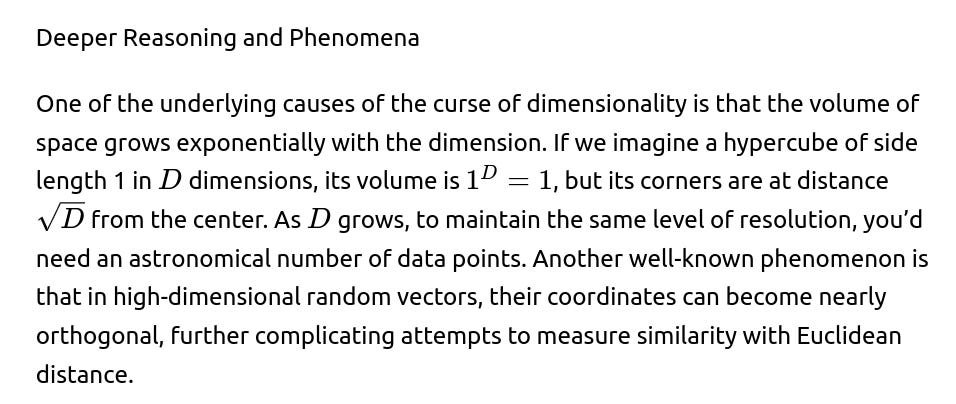
Why don’t extremely large datasets alone solve the curse of dimensionality?
Although collecting more data is generally beneficial, even extremely large datasets might not cover a high-dimensional space sufficiently. The volume of a D-dimensional hypercube grows exponentially with D. For instance, if you double the dimension, you typically need to square your data size to maintain the same density of coverage. This exponential growth quickly outpaces typical data collection capabilities. Another subtlety is that real-world data may concentrate in complex subregions or manifolds within the high-dimensional space, and random sampling might still leave large, critical parts of the manifold underrepresented. The problem of “sparsity in high dimensions” is fundamental. More data can help, but often domain insights, feature engineering, or dimensionality reduction are equally, if not more, crucial.
Additionally, the cost of labeling data may become prohibitive. You can collect a huge volume of unlabeled data, but supervised learning might still suffer if labeled data is only a small fraction. Active learning or semi-supervised techniques can help alleviate labeling costs, but they don’t fully circumvent the challenges posed by high-dimensional geometry.
How does PCA help in mitigating the curse of dimensionality, and what are its limitations?
PCA (Principal Component Analysis) projects data onto a smaller set of orthogonal directions that capture the largest variance in the dataset. By keeping only the top principal components, you discard directions of minimal variance. This can help in two ways:
It compresses the feature space into a lower dimension, potentially reducing computational and memory costs.
It removes noise-dominated directions, which can help distance-based methods find more meaningful neighborhoods in that lower-dimensional subspace.
However, PCA has limitations:
It only captures linear relationships. If your data lies on a highly non-linear manifold, PCA might not effectively represent the underlying structure.
It assumes that directions of high variance are the most informative for the target task. This may not always be true for classification or regression tasks in which class-discriminative directions can sometimes have smaller variance.
It is sensitive to outliers, which can skew the principal components if outliers produce abnormally large variance.
Non-linear dimensionality reduction methods like t-SNE, UMAP, Isomap, or using autoencoders can sometimes preserve local and/or global structure better. These approaches often give better performance on complex data manifolds. Still, they also can have significant computational overhead and parameter tuning complexities.
Are tree-based methods like Random Forests immune to the curse of dimensionality?
Tree-based methods such as Random Forests or Gradient Boosted Decision Trees often handle high-dimensional data more gracefully than simple distance-based methods, mainly because they partition the feature space using decision boundaries rather than explicitly depending on distance metrics. They also incorporate feature selection in a sense, as at each node split, a subset of features is considered. Over multiple trees, some relevant features can come to the forefront. But they are not entirely immune to the curse of dimensionality:
If there are many irrelevant features, the chance of random splits on those irrelevant features can lead to suboptimal splits or unnecessary complexity.
If the dimension is extremely high (with comparatively few samples), trees can still overfit or create very fragmented partitions.
Interpretability can degrade in very large feature spaces, and the model might depend on complex interactions that are not straightforward to understand.
Hence, while tree-based methods are often more robust compared to kk-NN or clustering in high dimensions, it’s still beneficial to apply dimensionality reduction, regularization, or feature selection to further improve performance and prevent potential pitfalls.
Below are additional follow-up questions
Can the curse of dimensionality be alleviated by standard normalization or standardization techniques alone? If not, why not?
Normalization or standardization (for example, subtracting the mean and dividing by the standard deviation for each feature) ensures that features are on a comparable scale. This often helps machine learning algorithms converge more quickly or prevents certain features from dominating. However, scaling alone does not fundamentally reduce the dimensionality or solve the issues caused by the exponential growth of the feature space. When dimensions are excessively large, distance-based calculations become less meaningful due to distance concentration. Simply rescaling each feature to a comparable range does not address the fact that there may be too many irrelevant or redundant dimensions for the model to discern genuine neighbors or patterns. So, while normalization is typically good practice, it is insufficient by itself to mitigate the root problems of the curse of dimensionality, such as the need for vastly larger datasets or the confusion in distance metrics when dimension grows high.
Potential Pitfalls: If one relies exclusively on standardization without performing feature selection or dimensionality reduction, the underlying sparsity and noise in high-dimensional data can remain. This might give a false sense of security because one sees well-scaled features, but the learned model might still generalize poorly or struggle to separate classes. Another subtle pitfall is that feature scaling can mask interactions or non-linear relationships, potentially requiring more advanced transformations or domain-specific feature engineering rather than pure normalization.
How does one handle the curse of dimensionality in streaming data scenarios, where data arrives incrementally and must be processed in real-time or near real-time?
In streaming data contexts, the model cannot rely on a one-time batch dimensionality reduction or an offline feature selection. Instead, the process must adapt to new data as it arrives. Techniques like incremental PCA, online random projections, or streaming autoencoders can update a lower-dimensional representation continuously without storing all past data. Using these incremental methods allows the system to efficiently maintain a compressed feature space. Additionally, one can employ online feature selection methods that dynamically assess the importance of features as new data arrives.
Potential Pitfalls: A real-time system may not accommodate slow or compute-heavy methods for dimensionality reduction, so practical constraints might force simpler approaches like incremental PCA or random projections rather than advanced manifold learning. If the data distribution shifts over time (concept drift), the previously chosen subspace or selected features may lose relevance. The system must incorporate drift detection and adaptation strategies to ensure that the representation remains aligned with the evolving data distribution. Failing to do so can degrade performance severely, especially in high-dimensional data streams where small changes can cascade into large errors.
In the context of dimension reduction, how do we ensure that the reduced dimension is still large enough to preserve the complex relationships needed by the model?
When applying dimensionality reduction (PCA, autoencoders, etc.), the challenge is to choose a dimension low enough to combat the curse of dimensionality, but still high enough to preserve essential information. One practical way to do this is to analyze reconstruction error or variance retention. For PCA, for instance, you might choose the number of components that captures a high percentage of the variance (e.g., 90% or 95%). In autoencoders, you might track reconstruction loss during validation. Additionally, you can track downstream performance metrics: if classification or regression performance declines sharply after reducing the dimension below a certain threshold, it might indicate that important structure was lost.
Potential Pitfalls: Stopping purely based on explained variance can be misleading. There might be directions in the data that explain little overall variance but are crucial for specific tasks (e.g., class-separability). Another pitfall is that manifold-based approaches can compress data in ways that preserve local geometry but lose global relationships. If the downstream task relies on global structure, the chosen technique or dimension might be suboptimal. Ensuring that cross-validation or hold-out validation is employed to confirm the adequacy of the dimensionality reduction is critical.
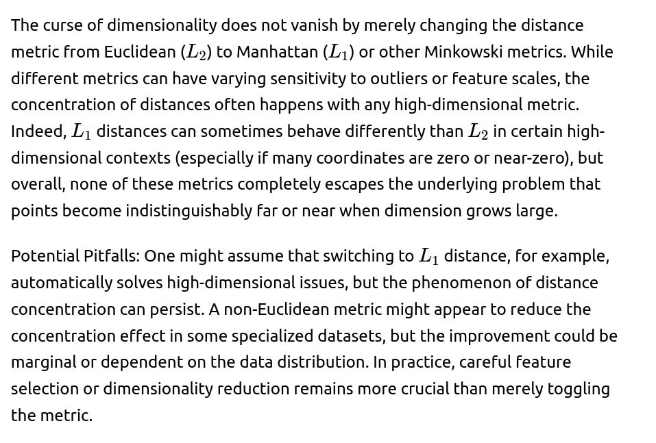
Could the choice of distance metric matter for the curse of dimensionality? For example, using Manhattan distance vs. Euclidean distance vs. Minkowski distance with different p values?
Are kernel methods immune from the curse of dimensionality or do they also suffer from it in certain contexts?
Kernel methods (like SVMs with the RBF kernel) implicitly map data into higher-dimensional feature spaces. At first glance, one might assume that kernel methods sidestep the curse of dimensionality by working in a possibly infinite-dimensional Hilbert space. However, they can still suffer if the original input dimension is very large and the data is not sufficiently numerous or well-structured. The model complexity of kernel methods can grow dramatically, requiring more support vectors to capture the decision boundary, which leads to high computational and memory costs. Also, if the kernel parameters (e.g., bandwidth in RBF) are not tuned properly, the model might overfit or underfit in high dimensions.
Potential Pitfalls: In very high-dimensional settings with limited data, kernel methods might pick many support vectors, leading to excessive runtime. Furthermore, hyperparameter tuning can become difficult as the dimension grows. If the kernel width (for RBF, often denoted γ or similar) is too large, the model might underfit by effectively flattening the decision surface; if it’s too small, it might overfit and memorize data points. The curse of dimensionality can thus manifest in the parameter-sensitivity and computational burden of the kernel approach.
How does the curse of dimensionality affect optimization-based learning methods that rely on gradient-based approaches (like deep neural networks)?
Deep neural networks do not explicitly rely on distance metrics in the same way k-NN or clustering methods do, but they can still be susceptible to the curse of dimensionality in several ways. High-dimensional input spaces often contain many irrelevant or redundant features that can confuse the gradient descent process, increasing the possibility of local minima or saddle points. Networks also become more prone to overfitting if regularization and data augmentation are insufficient. The data requirements for generalization may become massive; each training example only partially covers the high-dimensional input manifold.
Potential Pitfalls: Excessive dimensionality can cause exploding or vanishing gradients if the network architecture is not carefully designed or if the initialization is poor. Real-world aspects, such as limited labeled data for extremely high-dimensional tasks, frequently lead to over-parameterized networks that memorize training data. Regularization methods (e.g., dropout, weight decay) and advanced optimizers can help, but if the underlying dimension is too large, even neural networks with large capacity might fail to discover meaningful representations unless aided by domain knowledge, unsupervised pre-training, or carefully engineered architectures like convolutional layers in images or attention-based mechanisms in text.
How might the curse of dimensionality manifest differently in unstructured domains like images, text, or audio, where the input data is inherently high-dimensional, compared to tabular data with many columns?
Images, text, and audio naturally have many raw features (pixels, word embeddings, audio samples), yet deep learning architectures such as CNNs for images, Transformers for text, or convolutional/Recurrent networks for audio can capture local patterns or structure that mitigate the curse of dimensionality. For instance, convolutional layers exploit spatial locality by restricting receptive fields, effectively reducing the parameter space. Similarly, Transformers reduce the effective dimensionality by focusing attention selectively.
In contrast, tabular data may not possess strong spatial or temporal correlations, so local structures that can be exploited are often far less obvious. Feature interactions may be sporadic rather than systematically structured, making dimension reduction less straightforward. As a result, purely high-dimensional tabular data can be more problematic for distance-based methods and for neural networks not specialized to handle specific structures.
Potential Pitfalls: Even in unstructured data, if a naive approach is taken (e.g., flattening images into pixel vectors) without leveraging specialized architecture, the curse of dimensionality can strongly degrade performance. In text, if one uses extremely high-dimensional one-hot vectors rather than embeddings, the model can become very sparse and the number of features can grow unbounded. Carefully leveraging domain structure (local correlations, hierarchical relationships) is often vital to avoid drowning in large, unstructured feature spaces.
Does feature correlation reduce the effective dimensionality or does it still remain an issue for distance-based methods?
Strong correlations among features can reduce the effective dimensionality somewhat, because correlated features occupy a smaller subspace. For instance, if two features are perfectly correlated, they lie on a line in high-dimensional space. However, for distance-based methods, correlation does not necessarily protect against distance concentration. If the data distribution is spread out across several correlated axes, distance metrics can still degrade. Also, the presence of some correlations does not rule out the possibility that other dimensions remain sparse or uncorrelated.
Potential Pitfalls: Relying solely on correlation analysis might overlook non-linear relationships. Two features might be uncorrelated in a linear sense yet still contain overlapping information relevant to a predictive task (e.g., a non-linear correlation). A partial correlation among some dimensions might not counteract the complexity of many other independent dimensions. Thus, correlation alone typically does not solve the fundamental issues that come with large dimensionality.
Is there a possibility that ignoring or mishandling the curse of dimensionality can lead to ethical or fairness concerns in ML models?
When data is high-dimensional and models struggle to differentiate relevant from irrelevant features, spurious correlations or noise can creep into decision boundaries. This can inadvertently amplify biases. For instance, if a feature that correlates with a protected characteristic (like race or gender) inadvertently drives the model’s predictions due to high-dimensional overfitting, then the model could become discriminatory. Because dimensionality can obscure transparency—many features with small individual effects can combine into a large aggregated effect—biased outcomes can go unnoticed.
Potential Pitfalls: In fairness or bias auditing, one might fail to detect that high-dimensional effects are disproportionately harming certain subgroups. Mislabeled or under-represented data in high-dimensional space is even harder to spot or correct. If one does not properly mitigate the curse of dimensionality, the model might rely on these meaningless or biased signals. Hence, robust dimensionality reduction or thorough feature selection can be an integral step in building ethical ML systems.
How can one detect whether the curse of dimensionality is at play in a given dataset or if the performance issues arise from other factors?
The first sign might be a rapid degradation of performance in distance-based or generative models as dimension grows, even if the dataset size is large. Another indicator is that distance metrics begin to concentrate, which can be empirically tested by measuring the ratio of (minimum distance between points) to (maximum distance between points) and observing whether that ratio approaches 1. If it does, it suggests strong distance concentration. Visual inspection of pairwise distance distributions can also help. Another approach is to apply a dimensionality reduction method like PCA and see if a small number of components can explain most of the variance. If so, that suggests the data is effectively lying on a lower-dimensional subspace, and the apparent high dimensionality is partly “empty.”
Potential Pitfalls: Poor performance might not always be due to the curse of dimensionality. It could result from poor feature engineering, inadequate hyperparameter tuning, noisy data labels, or an inappropriate model architecture. Overemphasizing dimensionality as the single cause might lead one to overlook simpler explanations (like data preprocessing errors). Conversely, ignoring the high-dimensional structure could cause repeated attempts at “fixing” the model or hyperparameters that never address the real issue. A careful set of diagnostic tools—distance concentration tests, variance explained analysis, correlation heatmaps, domain understanding—helps disentangle the curse of dimensionality from other confounding factors.