ML Interview Q Series: After poor logistic regression performance, what improvements or alternative methods would you consider for better results?

📚 Browse the full ML Interview series here.

Short Compact solution

Features can be normalized so that no single feature scale dominates the model. If the current features seem insufficient, new and more discriminative ones can be added. Any outliers should be checked and dealt with properly, as they might skew the regression fit. You can also remove or keep certain variables if they introduce too much noise. A systematic approach like cross-validation, combined with hyperparameter tuning (for example, adding regularization), can help. If the dataset is not linearly separable, considering models such as SVMs, tree-based algorithms, or neural networks could yield improved results.

Comprehensive Explanation

Improving Logistic Regression Performance

Feature Scaling / Normalization Logistic regression often benefits from putting all features on comparable scales. When features vary widely in their magnitudes, the optimizer can take inefficient steps during gradient-based updates. Scaling can help gradient descent converge more smoothly, especially if you are using libraries that default to iterative solvers. It also ensures that no particular feature with large numeric range overshadows others.

Outlier Handling Outliers can disproportionately affect the logistic regression solution, especially if the model is sensitive to anomalies. Outliers might come from data collection or entry errors, or they might represent genuine rare events that deserve special treatment. You can investigate techniques like trimming extreme values, winsorizing, or applying robust methods that assign lower weight to extreme outliers.

Regularization and Hyperparameter Tuning Logistic regression has a built-in mechanism for regularization, such as L1 (Lasso) or L2 (Ridge). These can prevent overfitting by penalizing large weights. You can also adjust the regularization parameter (often denoted C in many libraries) to strike a balance between fitting the data and controlling model complexity. Coupling this with cross-validation helps in choosing optimal hyperparameters and assessing generalization performance.

Variable Selection Extra or irrelevant features sometimes introduce noise or increase the risk of overfitting. Selecting only the most pertinent features—either by domain knowledge, correlation analysis, or more formal methods like recursive feature elimination—can be beneficial. Regularized methods naturally perform a kind of feature selection: L1 regularization can drive certain coefficients to zero, discarding less important features.

Considering Alternative Models

When Data is Not Linearly Separable Logistic regression is a linear classifier:

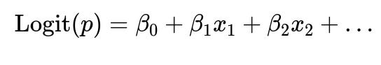
If the problem has a more complex decision boundary, linear logistic regression might struggle. Kernel-based SVMs, tree-based models (such as Random Forest or Gradient Boosting), or neural networks can capture more complex relationships.

Support Vector Machines (SVMs) SVMs, especially with non-linear kernels like the RBF kernel, can capture more complex boundaries. They can work well with high-dimensional datasets and can handle moderate data sizes effectively.

Tree-Based Methods Algorithms like Random Forest and Gradient Boosting (e.g., XGBoost, LightGBM) handle complex interactions and can naturally model non-linearities. They also often work well with unscaled data. They can provide insight into feature importances, helping guide further feature engineering.

Neural Networks Deep learning models are powerful for large-scale or highly unstructured data (images, text, etc.) but can also be used for tabular data. They can capture highly non-linear patterns if sufficient data and computational resources are available.

Ensemble Approaches Combining models (e.g., ensembling logistic regression with tree-based approaches) can sometimes improve performance, particularly if the models capture different aspects of the data distribution.

Follow-Up Questions

What factors determine whether feature normalization is required?

Feature normalization is particularly helpful if:

• The optimization algorithm uses gradient-based techniques that can become unstable with features of very different scales. • You suspect certain features with large magnitudes unduly influence the learning process. • You notice that hyperparameter tuning for regularized logistic regression becomes difficult because unscaled features skew the effect of regularization.

Edge cases to consider: • If your model is tree-based, scaling is generally less of a concern because tree splits are based on feature ordering. • If you have only a few carefully selected features that are on similar scales already, normalization might not yield noticeable gains.

How do you decide which new features to add?

You might:

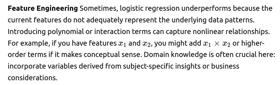
• Use domain expertise and brainstorming to hypothesize new data transformations or external data sources that might explain the outcome better. • Look at residual analysis to see if there's a pattern in predictions that might indicate missing interactions or non-linearities. • Check correlation with existing features and label: sometimes discovering new interactions or polynomial terms is guided by correlation heatmaps and partial dependence plots. • In some contexts, you can experiment with automated feature engineering libraries, but ideally, domain knowledge drives the choice.

How does outlier handling differ between logistic regression and, say, tree-based methods?

Logistic regression tries to fit a single linear decision boundary with a cost function often sensitive to extreme values. Large outliers can shift the decision boundary significantly or inflate certain coefficients. Tree-based methods, on the other hand, split on thresholds and are less influenced by extreme outliers because splits depend on the order of feature values rather than their magnitudes. This means tree-based models might be more robust when extreme values exist, though they still can be influenced by the presence of unusual data distributions.

Why does cross-validation help in hyperparameter tuning?

Cross-validation helps by:

• Splitting the dataset into multiple folds, ensuring you can repeatedly train and validate on different subsets of data. • Providing a more reliable estimate of how well your chosen hyperparameters generalize, since you are not fixing a single train/test split. • Reducing the chance of overfitting hyperparameters to a particular split, making your final model more robust.

When should one consider neural networks over logistic regression?

Neural networks can be valuable if:

• You have complex feature interactions that might not be captured easily by a simple linear model. • There is a large amount of data available. Neural networks often need substantial data to learn complicated patterns without overfitting. • The data is high-dimensional, unstructured, or includes images, text, or audio signals. Logistic regression has limited capacity in those domains, whereas deep networks can learn hierarchical representations from raw inputs.

Potential pitfalls: • Neural networks can overfit if you have insufficient data. • They require careful tuning of many hyperparameters (learning rate, number of layers, number of neurons, regularization, etc.). • They can be computationally expensive.

Could ensembling a logistic regression with more complex models be beneficial?

Yes, ensembling different algorithms often yields better performance than any single model alone because:

• Different models can learn complementary aspects of the data. • Logistic regression can provide a robust baseline or an interpretable portion of the ensemble, while a tree-based model or a neural network captures more complex patterns. • Stacking or blending these models can sometimes achieve lower variance and bias overall.

Edge cases: • Ensembling can lead to very large model sizes and more computational overhead in inference. • If interpretability is a priority, an ensemble can be less transparent, though you can maintain logistic regression separately for interpretability.

Is there a specific reason why logistic regression might fail other than linear separability?

Yes, a few key reasons include:

• Insufficient or irrelevant features: The model cannot learn a meaningful boundary if the predictors do not capture discriminative information. • Incorrect assumptions about feature relationships: Logistic regression expects a log-odds linear relationship. If real relationships are non-linear and not well-engineered, performance suffers. • Class imbalance: If one class is underrepresented, the model might become biased toward predicting the majority class. Techniques like class weighting or oversampling might be necessary. • Overfitting: If you have too many features and insufficient regularization, logistic regression can overfit, despite being relatively simpler compared to deep networks.

How do you handle class imbalance in logistic regression?

Techniques for class imbalance:

• Use class weights (e.g., in scikit-learn’s logistic regression) to penalize misclassifications in the minority class more heavily. • Oversample the minority class with SMOTE or random oversampling. • Undersample the majority class. • Combine sampling and class weighting for a more balanced performance. • Track additional metrics such as precision/recall, F1-score, or AUROC, rather than raw accuracy, to evaluate the model better.

If the imbalance is extreme, consider specialized approaches or even cost-sensitive methods where the logistic regression objective includes different penalty terms for false positives vs. false negatives.

How might you implement a basic logistic regression model with regularization in Python?

Below is a simple example using scikit-learn:

import numpy as np
from sklearn.model_selection import train_test_split, GridSearchCV
from sklearn.linear_model import LogisticRegression
from sklearn.metrics import accuracy_score

# Suppose X, y are your features and labels, respectively
X_train, X_test, y_train, y_test = train_test_split(X, y, test_size=0.2, random_state=42)

# Simple logistic regression with L2 regularization
model = LogisticRegression(penalty='l2', solver='liblinear', C=1.0)  # C is the inverse regularization strength
model.fit(X_train, y_train)

# Predictions
y_pred = model.predict(X_test)
print("Accuracy:", accuracy_score(y_test, y_pred))

# Hyperparameter tuning with GridSearchCV
param_grid = {
    'C': [0.01, 0.1, 1, 10, 100],
    'solver': ['liblinear', 'lbfgs']
}
grid_search = GridSearchCV(LogisticRegression(penalty='l2'), param_grid, cv=5, scoring='accuracy')
grid_search.fit(X_train, y_train)

best_model = grid_search.best_estimator_
print("Best parameters:", grid_search.best_params_)
print("Best CV accuracy:", grid_search.best_score_)

The parameter “C” controls regularization strength (lower values indicate stronger regularization). By tuning it via cross-validation, you balance underfitting and overfitting.

Below are additional follow-up questions

How does one deal with multicollinearity among features in logistic regression, and why is it problematic?

Multicollinearity occurs when two or more input variables are highly correlated. In logistic regression, this is problematic because the model tries to fit coefficients to variables that essentially carry overlapping or redundant information. In practice, this causes the coefficient estimates to become unstable or extremely large in magnitude, which can produce numerical instability and inflated variance in the parameter estimates.

To address multicollinearity:

• Regularization Methods Ridge (L2) regularization often helps control excessive coefficient swings by penalizing the sum of squared coefficients. By shrinking coefficients, it reduces the impact of correlated features. Lasso (L1) regularization can push some coefficients to zero, effectively performing feature selection. Pitfall: If you use Lasso alone, one correlated feature might be zeroed out while the other is retained. This can complicate interpretability if you rely on which feature is “zeroed out.” If both features are equally valid, the model might keep one arbitrarily while discarding the other.

• Dimensionality Reduction Techniques like PCA or SVD can transform correlated features into orthogonal (uncorrelated) components. You then train logistic regression on those components. Pitfall: Although PCA can alleviate collinearity, it makes interpretability more difficult because the new components no longer map directly to original features.

• Feature Elimination If domain knowledge indicates that two features are highly correlated, you might remove one. Pitfall: Removing features based solely on correlation thresholds can cause accidental loss of important nuanced information if you aren’t careful.

• Domain-Based Approach Sometimes domain knowledge helps unify overlapping features. For example, you might compute a new feature that is some meaningful combination of the correlated variables. Pitfall: This requires thorough domain knowledge. A naive combination might worsen the problem or lose predictive power.

What if you have a streaming or online learning scenario where new data arrives continuously?

When data arrives as a stream, you often cannot afford to retrain from scratch each time. You need an online or incremental learning approach to update model parameters in small steps as new data arrives.

• Stochastic Gradient Descent (SGD) Logistic regression can be trained incrementally using SGD. Each new data instance (or mini-batch) updates the coefficients. Pitfall: Learning rates must be chosen carefully. Too large leads to divergence; too small leads to extremely slow convergence.

• Data Drift Detection Over time, the underlying distribution may shift (concept drift). Periodically evaluate model performance on incoming batches and compare with historical metrics. If performance degrades significantly, consider re-initializing your online learning algorithm or adjusting the learning rate. Pitfall: Continual updates without drift detection can cause the model to over-correct based on outlier segments of data, resulting in worse overall performance.

• Memory and Computational Constraints Online learning is often chosen to cope with memory limits; you only maintain a small buffer of data. Pitfall: Improper buffering (e.g., storing too large a window of recent data) can negate the main advantage of streaming approaches.

How does logistic regression handle noisy or mislabeled data, and what are potential mitigation strategies?

Noisy or mislabeled data can mislead the logistic regression model. Because logistic regression tries to fit a decision boundary consistent with all labeled examples, mislabeled instances can pull the boundary in the wrong direction.

• Robust Loss Functions Traditional logistic regression uses the log loss, which can be sensitive to extreme mislabels. Some robust variants of logistic regression alter or reweight the loss function to reduce the impact of suspicious data points. Pitfall: Implementing custom robust loss can be non-trivial. Also, if you over-penalize potential outliers, you might throw away genuinely correct, rare data points.

• Data Cleaning and Preprocessing Often the most direct approach is to identify and correct or remove clearly mislabeled samples. This can be done via outlier detection or cross-checking with domain experts. Pitfall: Automated detection of mislabeled data is itself error-prone, especially if the data truly has unusual but valid cases.

• Confidence-Based Filtering If the model consistently assigns extremely low probability to a label for a data point, it might indicate a possible mislabel. You can re-check or temporarily remove such points. Pitfall: This approach depends on the current model’s reliability. If your initial model is poor, it might incorrectly flag legitimate data as mislabeled.

How can logistic regression be adapted to multi-class classification problems beyond the binary setting?

While logistic regression is inherently binary, it can extend to multi-class scenarios using strategies like “One-vs-Rest” (OvR) or “Multinomial Logistic Regression” (also called Softmax Regression).

• One-vs-Rest (OvR) You train multiple separate binary logistic regressions, each discriminating one class from all others. The class whose model outputs the highest positive score (or probability) is chosen. Pitfall: OvR can produce inconsistent probability estimates across different class models. Additionally, you end up training K models for K classes, which can be computationally heavier.

• Multinomial Logistic Regression (Softmax) This single model generalizes logistic regression to predict probabilities across K classes with a softmax function. It ensures that all class probabilities sum to 1. Pitfall: If K is extremely large (like thousands of classes), the softmax might become computationally intense. You might consider approximate methods or hierarchical softmax.

• Hierarchical Approaches If you have a natural structure among classes (e.g., categories and subcategories), you can do a tiered classification pipeline. Pitfall: Errors in the first tier can propagate, causing the final classification to fail if the hierarchy is not well-defined or data in one branch is significantly less than another.

  When is it advantageous to use a penalized likelihood approach (e.g., Bayesian Logistic Regression) instead of standard frequentist logistic regression?

  Bayesian logistic regression places priors on model parameters, leading to posterior distributions rather than point estimates. This is beneficial when:

  • Uncertainty Quantification Bayesian methods naturally provide distributions for the coefficients, allowing you to quantify uncertainty about each parameter. Pitfall: Full Bayesian inference can be computationally expensive. Sampling methods (e.g., MCMC) might not scale well with large datasets.

  • Limited Data Scenarios If you have small or noisy datasets, imposing priors can prevent extreme parameter estimates. Pitfall: Choosing the wrong priors can hurt performance if they conflict with the true data distribution.

  • Interpretability of Parameter Distributions You can see how certain or uncertain the model is about each coefficient. This can be crucial in applications like medicine or finance. Pitfall: The interpretability advantage depends on stakeholders being comfortable with probabilistic reasoning. If they prefer a single estimate rather than a distribution, Bayesian benefits might be underused.

  How might you approach model interpretability concerns in logistic regression?

  Logistic regression is often considered interpretable because each coefficient has a direct relationship to the log-odds of the outcome. However, real-world nuances can complicate this:

  • Standardized Coefficients When features have different scales, you can standardize them so that coefficient magnitudes become more comparable. Pitfall: Standardizing can obscure the original units of the features, making direct domain interpretation less intuitive.

  • Interaction Terms If you introduce interaction or polynomial terms, interpretation becomes more complex, as coefficients now reflect the combined effect of multiple features. You might have to use partial dependence plots to see the effect of specific feature interactions on predicted probability. Pitfall: Overuse of interaction terms can undermine the primary advantage of logistic regression’s simplicity and interpretability.

  • Model Explanation Tools Techniques like LIME or SHAP can be applied even to logistic regression for local or global explanations. They confirm whether your intuition about coefficients aligns with the model’s local predictions. Pitfall: If your dataset is extremely large or high-dimensional, even these tools can become computationally expensive.

  What if your dataset is extremely large and doesn’t fit into memory for logistic regression?

  Large-scale data can pose serious challenges:

  • Incremental or Online Learning Similar to the streaming scenario, you can apply an incremental learning approach where you process data in chunks. Pitfall: If you pick too large a batch, you might still face memory constraints. If you pick too small a batch, you risk very noisy gradient estimates.

  • Distributed Training Libraries like Spark MLlib or parameter-server frameworks can distribute logistic regression across multiple machines. Pitfall: Communication overhead can become a bottleneck. Also, distributed setups can be complex to maintain and debug.

  • Mini-Batch Approaches with SGD A typical approach is to read from disk in mini-batches and update model parameters. Tools such as PyTorch’s DataLoader can handle mini-batch generation. Pitfall: Tuning the learning rate schedule is critical. A bad schedule can degrade performance, especially with massive data volumes.

  How do you determine the optimal threshold for classification in logistic regression if your application demands a certain precision or recall?

  Although logistic regression outputs a probability, the default threshold for converting probabilities to class labels is often 0.5. This might not be optimal for certain metrics or business needs.

  • Precision-Recall Trade-offs If you need high precision (few false positives), raise the threshold so that only high-confidence predictions are labeled as positive. Conversely, if you need higher recall (catch more positives), you might lower the threshold. Pitfall: Overly increasing threshold to boost precision might severely reduce recall. In a medical test scenario, missing positives could be a bigger issue than having false positives.

  • Cost-Sensitive Thresholding You might define a custom cost function that quantifies the cost of false positives vs. false negatives. Then you can search for the threshold that minimizes overall expected cost on a validation set. Pitfall: Determining real-world costs can be subjective or based on assumptions that change over time.

  • Calibration Curves and ROC Curves By examining metrics like the ROC curve (TPR vs. FPR) or Precision-Recall curve, you pick a threshold that balances the trade-off that best suits your application. Pitfall: If the data has a strong class imbalance, sometimes the ROC curve can be misleading. Precision-Recall curves are more informative in such cases.

  In what cases might you want to transform the target variable before performing logistic regression?

  Normally, logistic regression is applied to a binary target (0 or 1). However, there are scenarios where the raw target might need transformation:

  • Ordinal Logistic Regression If you have ordered categories (like star ratings 1–5), you might move to ordinal logistic regression so that the model leverages the ordinal relationship. Pitfall: The assumption that the distance between adjacent levels is consistent (e.g., the difference between ratings 1 and 2 is the same as between 4 and 5) might not hold in practice.

  • Grouped or Aggregated Data Sometimes you have data counts (number of successes vs. number of trials) rather than individual binary labels. You can use a binomial logistic regression approach that accounts for the group size. Pitfall: If group sizes vary wildly, you need weighting. A group with 100 trials vs. a group with 2 trials can influence the model differently.

  • Label Encoding In multi-class scenarios, a naive label encoding (0,1,2,3,...) doesn’t necessarily reflect any meaningful numeric relationship. You must use one-hot encoding or other methods rather than feeding numeric labels directly. Pitfall: Misapplication of numeric encodings to categorical variables in logistic regression can cause the model to interpret them as ordinal, leading to incorrect relationships.

  How does logistic regression handle missing values, and what are some strategies to manage them?

  Logistic regression does not inherently handle missing values. Traditional implementations like scikit-learn’s LogisticRegression require no missing entries.

  • Imputation Common strategies include mean, median, or most-frequent-value imputation. More sophisticated approaches involve using predictive models to fill missing entries. Pitfall: Simple imputation can bias the data if the missingness is not random. Predictive imputation can lead to “leakage” if done incorrectly (i.e., using target information to impute features).

  • Indicator Variables One technique is to create a binary variable indicating whether a value is missing or present, then impute a default. Pitfall: This might artificially separate the data if the reason for missingness is not relevant or if it correlates strongly with the target.

  • Model-Based Approaches Some libraries support logistic regression with specialized missing data handling, such as MICE (Multiple Imputation by Chained Equations). This systematically draws plausible values for missing data. Pitfall: These methods can be computationally heavy and rely on assumptions about the missing data mechanism (Missing Completely at Random, Missing at Random, etc.).

  How might you validate a logistic regression model if your data is time-dependent?

  If data has temporal structure (e.g., forecasting future events), random splits can lead to data leakage because future data might appear in the training fold. Proper temporal splits are essential:

  • Rolling Forecast Origin Train the model on data up to time tt, then validate on time t+1. You continue “rolling” this forward. Pitfall: It can reduce the amount of training data for each split and might increase variance in your validation metrics.

    Block Cross-Validation Partition the time series into contiguous blocks, ensuring the training block precedes the validation block. Pitfall: Overlapping or non-overlapping blocks both have trade-offs. Non-overlapping blocks can waste data; overlapping blocks complicate independence assumptions.

  • Beware of Feature Leakage Ensure that any feature engineering using future data (such as lag features or moving averages) is done strictly within training intervals. Pitfall: If you use a window that extends beyond the training period to compute a moving average, you inadvertently leak future information into the training set.

  Under what circumstances might logistic regression coefficients become numerically unstable or fail to converge?

  Certain conditions can cause instability or non-convergence:

  • Perfect Separation If a combination of features can perfectly separate the classes, the maximum likelihood solution leads some coefficients to tend to infinity. Pitfall: Perfect separation might happen with small datasets or extremely strong predictor variables. The model might not converge using standard solvers.

  • Too Large a Learning Rate (in Gradient-Based Approaches) If you are using gradient descent or stochastic gradient descent, an excessively large step size can cause the updates to diverge. Pitfall: The model’s loss might not consistently decrease. You might see oscillating or exploding coefficient values.

  • Data Scaling Issues Extremely large feature magnitudes might produce large gradients or cause numerical overflow in the exponential function inside the logistic function. Pitfall: Even small changes in the features can lead to drastic coefficient changes, making training unstable.

  • Multi-Collinearity As mentioned earlier, highly correlated features can inflate some coefficients, making them numerically large even if changes in the data are small. Pitfall: Without regularization, collinearity can produce extremely large standard errors and hamper interpretability.

  • Inadequate Regularization If the model is complex or the dataset is noisy, you might need L1 or L2 regularization to stabilize parameter estimates. Pitfall: Too little or no regularization can allow coefficients to blow up; too much can degrade model performance by underfitting.