ML Interview Q Series: Amoeba Extinction Probability: A Branching Process Fixed-Point Solution.

Browse all the Probability Interview Questions here.

Imagine you have a jar with one amoeba at the start. Every minute, that amoeba (and all subsequent amoebas) can, with equal probability of 1/4, die, remain unchanged, split into two, or split into three. Determine the probability that the population eventually becomes extinct.

Short Compact solution

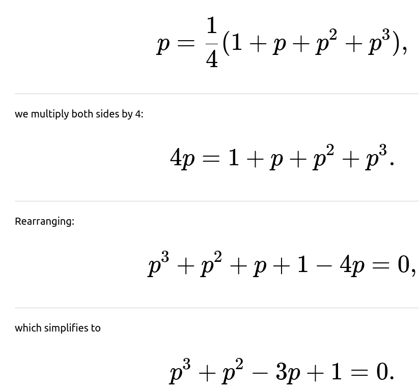
Let p be the probability that the jar’s amoebas eventually die out entirely. Because the process is the same at each minute, p also represents the probability of extinction after one minute and beyond. By conditioning on the single amoeba’s possible outcomes at the next minute:

Comprehensive Explanation

The process described can be viewed as a branching process, where each amoeba independently produces 0 (dies), 1 (unchanged), 2, or 3 offspring in the next generation with equal probability. The main idea is to identify p as the probability of eventual extinction starting from exactly one amoeba. Because the behavior is memoryless and each new amoeba follows the same probabilistic rules, the extinction probability is the same no matter which minute we observe the population.

The fundamental equation arises by conditioning on the first minute’s events. In more detail:

• If the amoeba dies (probability 1/4), the process ends in extinction for certain in that scenario.

• If the amoeba does nothing (probability 1/4), we are still left with exactly one amoeba, which has extinction probability p.

The importance of restricting ourselves to a solution in [0,1] comes from interpreting p as a probability. Any real roots outside this range do not make sense as probabilities for extinction. This process—also sometimes referred to as a Galton-Watson branching process—has an expected number of offspring per amoeba that is:

Follow-up question: How do we solve the equation in detail?

Solving the cubic equation can be done by standard algebraic manipulations:

Starting from

Follow-up question: Why is this a branching process, and how does that viewpoint help?

In a branching process interpretation, each individual amoeba acts as a “parent” that produces a random number of “offspring.” In this scenario, each parent produces 0, 1, 2, or 3 offspring with probability 1/4 each. The benefit of viewing it as a branching process is that it allows us to use powerful theorems and well-known approaches, such as generating functions, to analyze extinction probabilities. By letting the generating function be

the extinction probability is the unique fixed point of G(s) in [0,1]. This connection simplifies the analysis of more complicated branching settings and is a standard tool in stochastic processes.

Follow-up question: Could we simulate this in Python to verify?

Yes, we can. A straightforward Monte Carlo simulation repeatedly executes the rules for some large number of trials to approximate the extinction fraction. Below is an example using Python:

import random
import numpy as np

def simulate_amoeba_process(num_simulations=10_000_00):
    extinct_count = 0

    for _ in range(num_simulations):
        # start with a list representing one amoeba
        amoebas = [1]
        while amoebas:
            new_generation = []
            for _ in amoebas:
                event = random.randint(1, 4)  # each equally likely
                if event == 2:
                    new_generation.append(1)
                elif event == 3:
                    new_generation.extend([1, 1])
                elif event == 4:
                    new_generation.extend([1, 1, 1])
                # event == 1 means it dies, so we do nothing

            amoebas = new_generation
            # To prevent infinite loop in extremely large growth,
            # we could add a max iteration check if needed

        extinct_count += 1

    return extinct_count / num_simulations

prob_extinction_est = simulate_amoeba_process()
print("Estimated probability of extinction:", prob_extinction_est)

In this code:

We track the colony as a list of amoebas (each represented by a dummy value, like 1). Each minute, we simulate each amoeba’s action (die, stay, split into 2, or split into 3), and compile the new generation. We check when the list becomes empty, signifying extinction. After many simulations, the fraction of runs that end with no amoebas approximates p.

Follow-up question: Why is the probability less than 1, even though the expected offspring is 1.5?

When the reproduction rate (mean offspring) is above 1, it indicates that on average the population grows. However, randomness can still lead to early terminations in some fraction of the outcomes. The population either explodes to large numbers or dies out, and there is a certain probability of dying out that is strictly less than 1. This is a hallmark of supercritical branching processes where mean offspring per parent exceeds 1 but extinction still occurs with some probability.

Follow-up question: Are there any edge cases or special scenarios?

One potential edge case is if the probabilities of offspring had been modified so that the expected number of offspring is at or below 1. For instance:

If the expected offspring is exactly 1, the process is called critical, and the extinction probability often becomes 1 (unless there is a degenerate case with offspring distribution). If the expected offspring is below 1, the process is subcritical, and extinction becomes a certainty (probability 1). If the expected offspring is very large, there is still always some positive probability that the lineage will die out at some point, though that probability becomes smaller.

In this specific scenario with probabilities all equal to 1/4, the average is 1.5, so we label it supercritical, and hence the extinction probability is strictly between 0 and 1.

Below are additional follow-up questions

What if the probabilities of each outcome (die, do nothing, split into two, split into three) are not all equal?

A key subtlety arises in determining which root of the resulting polynomial lies in the [0,1] range. There can be multiple real solutions, but only one valid probability. In an interview, one might be asked to outline how to identify the physically meaningful solution and why extraneous real solutions are discarded.

How does the extinction probability change if we introduce a time limit?

What if the behavior of each amoeba is correlated, rather than independent?

In a correlated setting, you would need to model the joint behavior of all amoebas in each generation. This typically involves a more complex Markov chain or a more intricate state-based approach with a larger state space (tracking how many amoebas are alive at once and possibly their correlation structure). The generating function approach might not directly apply. One possible approach is to specify a joint probability distribution over the total number of children produced by the entire population at each step, rather than per-amoeba. This is conceptually more difficult and is prone to combinatorial explosion in the number of states.

How do we handle partial observations, such as only observing the total population size rather than each amoeba’s fate?

A major difficulty here is that different branching parameter combinations can lead to very similar population evolutions (identifiability concerns). Also, if the population is large, we might have limited data about individual events. Advanced methods like Markov chain Monte Carlo (MCMC) could be used to infer the distribution over possible parameter values. Once we have an estimated model, we can then compute an estimated extinction probability.

This is a subtle challenge because partial observability generally introduces extra uncertainty, and the extinction probability calculations might come with confidence intervals or require repeated sampling from the posterior distribution.

Could there be a scenario where amoebas have a carrying capacity or resource limit?

Yes. In reality, resources such as food or space might cap the total population. Once the population reaches a certain level, the probability of splitting might decrease, or the probability of dying might increase. This changes the problem from an unbounded branching process to a birth-death process with a maximum capacity. The extinction probability can still be computed in principle, but the underlying transition structure is more complicated:

• States represent the current number of amoebas.

• There are transitions from state n to states n−1, n, n+1, or n+2, depending on how many amoebas decide to die or split.

• Once n reaches the carrying capacity K, the splitting probabilities or outcomes might differ (e.g., forced to remain at K or forced to kill off some fraction).

This becomes a finite-state Markov chain, where eventual extinction probability can be determined by finding the probability of hitting state 0 before returning repeatedly to higher states. Techniques like solving systems of linear equations for hitting probabilities or using matrix methods can be employed.

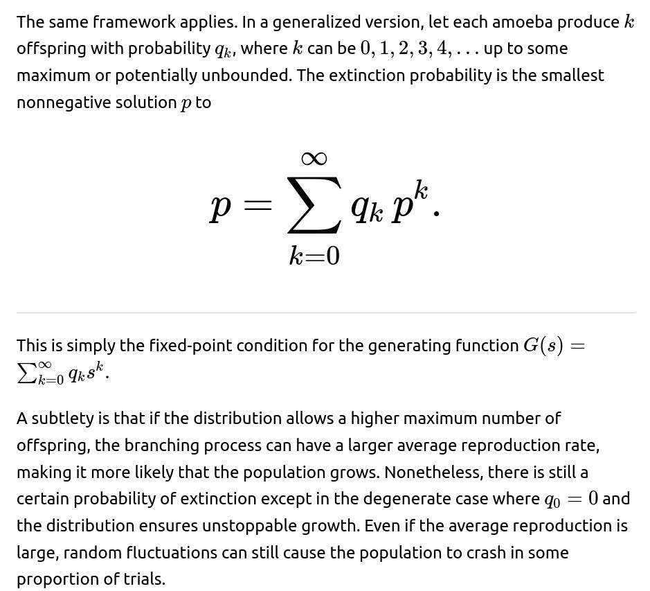
What if the amoeba splits into more than three offspring, or there are additional states like splitting into four or five?

How would we incorporate continuous-time models where splitting might occur at random intervals, not discrete minutes?

For a continuous-time process, each amoeba might have an exponential or some other waiting time distribution until it splits or dies. This is modeled by branching processes in continuous time, often called a birth-death process if the maximum offspring is one, or a more general Markov branching process if multiple offspring are possible. The main difference is that transitions now occur at random continuous times rather than fixed discrete steps.

To find extinction probabilities, we still rely on a generating function approach. The difference is that the generating function evolves according to differential equations rather than discrete recursion. The ultimate extinction probability is still the smallest nonnegative root of the steady-state equation p=G(p), where G is the generating function describing the distribution of total offspring for a single amoeba over its lifetime.

How can numerical stability issues arise in solving for p computationally?

Practitioners often mitigate this by using specialized numeric methods (like Newton-Raphson or bisection) and bounding the solution within [0,1]. One also checks the final solution carefully by plugging it back into the generating function to see if ∣G(p)−p∣ is near machine precision. In interviews, highlighting awareness of such practical details shows strong real-world experience.

Could the same approach be used if the jar initially contained multiple amoebas?

A nuanced point arises if the initial n amoebas are somehow correlated in their behavior or if they influence each other’s probabilities, in which case you cannot simply exponentiate. In typical branching process frameworks, independence is assumed unless otherwise specified.