
ML Interview Q Series: Analyzing a Two-Player Probability Game with Geometric Random Variables and Tie Advantage.

Browse all the Probability Interview Questions here.
9E-29. You and your friend both draw a random number from {1,2,…,10} at the same time and independently of each other. This procedure is repeated until you have drawn one of the four numbers {1,…,4} or your friend has drawn one of the six numbers {5,…,10}. The first player to get one of his marked numbers is the winner with the convention that you are the winner if a tie occurs.
a. What is your probability of winning the game? b. What is the probability mass function of the length of the game?
Short Compact solution
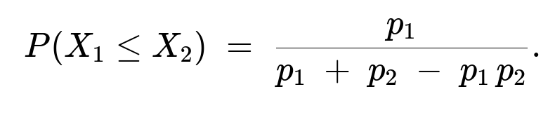
Define X1 as the number of draws you need to get a number from {1,2,3,4}, and X2 as the number of draws your friend needs to get a number from {5,6,7,8,9,10}. Let p1 = 4/10 and p2 = 6/10 be the respective probabilities of “success” in a single draw for you and your friend. Then the event “you are the winner” occurs if X1 <= X2. A direct calculation yields

Substituting p1 = 4/10 and p2 = 6/10, we get P(X1 <= X2) ≈ 0.5263.
The length of the game is min(X1, X2). It can be shown that min(X1, X2) follows a geometric distribution with parameter p = p1 + p2 − p1 p2 = 0.76. Hence,

so the probability mass function of min(X1, X2) is geometric with p = 0.76.
Comprehensive Explanation
Defining the random variables
To analyze who wins and how long the game lasts, we define two geometric-type random variables:
X1: The number of draws needed for you to get a number from {1,2,3,4}.
X2: The number of draws needed for your friend to get a number from {5,6,7,8,9,10}.
Each draw is from the discrete uniform distribution over 1 to 10. On each draw:
You succeed (i.e., draw one of {1,2,3,4}) with probability p1=4/10.
Your friend succeeds (i.e., draws one of {5,6,7,8,9,10}) with probability p2=6/10.
Because both of you draw simultaneously and independently, the trials for X1 and X2 can be viewed as independent geometric processes with their own success probabilities p1 and p2, respectively.
Probability of winning
The rule that you win in the event of a tie implies that “you win” is the event X1 <= X2. The key insight is to compute:
P(X1 <= X2) = P(X1=1, X2≥1) + P(X1=2, X2≥2) + ...
But a neater way is to use the fact that:
P(X1 <= X2) = ∑[j=1 to ∞] p1(1−p1)^(j−1) * P(X2 ≥ j).
Since X2 is geometric with probability p2, we have P(X2 ≥ j) = (1−p2)^(j−1). Multiplying these out and summing, we get a known closed form:
Plugging in p1=0.4 and p2=0.6 yields approximately 0.5263, which is indeed greater than 0.5.
Intuitive reason why your probability is above 0.5
It might initially seem surprising that you have a higher than 50% chance of winning even though your friend has the bigger set {5,...,10} of size 6. However, you also benefit from the rule that a tie goes to you. Whenever both of you draw your respective marked numbers on the same trial, you automatically win. This tie-break advantage effectively boosts your overall winning probability above 50%.
Distribution of the game length
The length of the game is the first time either of you draws a “success.” In random variable notation, the length is min(X1, X2). For min(X1,X2) to be greater than l, it means that both X1 and X2 are greater than l. Since X1 > l occurs with probability (1−p1)^l and X2 > l occurs with probability (1−p2)^l, and these events are independent, we get:
P(min(X1,X2) > l) = (1−p1)^l (1−p2)^l = (1−p)^l,
where p = p1 + p2 − p1 p2 = 0.76.
From this survival-function-based reasoning, the probability that min(X1,X2)=l is:
Thus min(X1,X2) is a geometric random variable with parameter p = 0.76.
Practical interpretation
On each draw, there is a combined probability p=0.76 that the game ends (because either you or your friend or both draw a successful number). Equivalently, there is a 24% chance the game continues after any given draw.
The probability that the game ends on the l-th draw is 0.76 × (0.24)^(l−1). So most games end relatively quickly (in just a few draws) given the relatively large combined probability of success on each draw.
Your winning probability is a bit above 0.52, reflecting the tie-break advantage.
Potential Follow-Up Questions
How does the tie-breaking rule influence the final probability?
The key role of the tie-breaking rule is that whenever both you and your friend draw your respective marked numbers on the same trial, you are declared the winner. Without that rule, we would have P(X1 < X2) instead of P(X1 <= X2). In that scenario, the probability would be strictly less than 0.5, because your friend has a higher single-draw success rate (0.6 vs. 0.4). The tie break in your favor shifts the probability above 0.5.
Does the geometric nature of X1 and X2 guarantee the game ends almost surely?
Yes. Since each draw has a positive probability (0.76) that the game will end (either you or your friend succeeds), the probability that it continues forever is zero in theory. In practice, the probability that the game is not decided by the l-th draw decreases exponentially fast in l.
Could the sets {1,2,3,4} and {5,6,7,8,9,10} overlap in a different scenario?
If the sets overlapped or changed in size, we would have different success probabilities for you and your friend. One would need to recalculate p1 and p2 accordingly. The same formula for P(X1 <= X2) with tie going to you would still hold if p1 and p2 represent the correct probabilities for each draw, but the numeric value would change based on the sets.
How might this relate to machine learning experiment design?
In some multi-armed bandit or reinforcement-learning settings, we analyze “success probabilities” for different strategies or arms. Though not exactly identical to a repeated uniform draw, the idea of repeated independent trials with different success probabilities is reminiscent of simpler RL or bandit problems. Also, this problem demonstrates how tie breaks and rules around “which event is considered success” can shift outcome probabilities.
Could we extend this reasoning to more players or different sets?
Yes, the same approach generalizes. If multiple players each have distinct success probabilities p1, p2, p3, etc., one can look at the random variables X1, X2, X3, etc., representing the first success for each player. The distribution of min(X1, X2, X3, ...) is still geometric with parameter (p1 + p2 + p3 + ... - any intersection terms). Determining who wins if there’s a tie can get more involved, but it’s manageable with careful enumeration or the law of total probability.
Below are additional follow-up questions
If the random draws were from a non-uniform distribution, how would we compute the winning probability?
If each draw were not equally likely to be any number from 1 to 10—for example, if some numbers had higher chance than others—we would need to recalculate the success probabilities p1 and p2 for you and your friend. Specifically, define p1 to be the probability of drawing any of {1,2,3,4}, and p2 to be the probability of drawing any of {5,...,10}, under the new non-uniform distribution. The overall structure of the solution remains:
X1 is still geometric with success probability p1, but p1 must be computed by summing the probabilities of drawing each of your desired numbers in one trial.
X2 is geometric with success probability p2, computed similarly for your friend.
The event “you win” is X1 <= X2 (tie goes to you).
The probability that you win still has the same form p1 / (p1 + p2 - p1 p2), but only if these p1 and p2 truly represent independent success probabilities in each draw.
The length of the game min(X1,X2) is geometric with parameter p1 + p2 - p1 p2 if each trial for both players is still independent across time.
Potential pitfalls:
If the distribution for each draw changes over time, p1 and p2 must be adjusted per draw. We cannot simply assume the same p1 and p2 for all trials.
If your distribution and your friend’s distribution are correlated (e.g., one number is more likely to appear only if another certain number has appeared), independence breaks down and invalidates the direct product approach.
How would the result change if only a finite number of draws is allowed?
In a real-world scenario, we might say the game stops after at most N draws. Then there is a possibility that neither you nor your friend draws a “successful” number within those N attempts. We would have:
A non-zero probability that the game ends in neither side’s favor (if it’s forced to stop at N). So we’d have to redefine the rules for what happens if no one succeeds by the N-th draw.
P(X1 <= X2) might be conditioned on the event that “someone eventually succeeds within N draws.”
To compute your overall chance of winning:
Compute the probability that X1 <= N or X2 <= N. If it is possible that both exceed N, then that leftover probability might be allocated to “no winner” or “incomplete game.”
Within the range 1 to N, carefully sum P(X1=j, X2>j) plus the probability of ties.
The distribution of min(X1,X2) would no longer be purely geometric because it is truncated at N. Hence you would have a truncated geometric distribution for the game length.
Potential pitfalls:
Forgetting to handle the leftover probability that min(X1,X2) > N leads to incorrect normalization.
If the game terminates with a different fallback rule (e.g., “everyone loses” if no success by the N-th draw), the final probability must account for that scenario.
What if, instead of a tie going to you, the tie triggers a new tiebreaker draw?
In this alternative rule, if both of you succeed in the same round, you go to a special “tiebreaker” procedure. This changes the probability that you win on any given round.
Let q = P(both succeed on a particular draw) = p1 p2, because draws are independent.
With the original tie-to-you rule, that probability q effectively contributes entirely to your win.
If the tie triggers a new tie-breaking sequence, the final distribution of winners depends on what that tiebreaker process looks like. For instance, if the tiebreaker is a fair coin, the fraction of q that translates to your ultimate win is 0.5 instead of 1.
You would then need to recalculate your overall winning probability, factoring in repeated tie events or the probability that the tiebreaker itself might not be decisive on the first attempt.
Potential pitfalls:
The tiebreaker might itself involve repeated draws or a separate random process with different probabilities. This can turn the entire event into a more complicated stochastic process.
If tie events can happen multiple times, you would have to consider an infinite geometric-like series of possible ties and their resolutions.
How does the assumption of independence between your draws and your friend’s draws affect the probability calculation?
The derivation of P(X1 <= X2) relies on your draws being independent of your friend’s draws. If these draws were correlated—for instance, if the outcome of your friend’s draw somehow influences your outcome—then we cannot simply multiply or sum the probabilities p1 and p2 in the same way.
In a dependent scenario, the probability that both you and your friend succeed on the same draw might no longer be p1 p2. It could be larger or smaller depending on the nature of the correlation.
The formula p = p1 + p2 - p1 p2 for the probability that at least one succeeds in a single draw might no longer hold, because that formula depends on independence.
Potential pitfalls:
Overlooking subtle dependencies in a real system (e.g., if one set of numbers is more likely to appear than another depending on external conditions) can completely change the results.
Even a small correlation could shift the overall probability of a tie or single-person success.
What if only one success event can occur in a single draw?
Imagine a revised game where once a number from {1,2,3,4} appears, it cannot also be considered a success from {5,...,10} in the same draw. This means that if a number in {1,...,4} comes up, it is physically impossible for {5,...,10} to appear at the same time. This would effectively make the events “you succeed” and “your friend succeeds” mutually exclusive on a single draw.
If the events are mutually exclusive, then p = P(either you succeed or friend succeeds) = p1 + p2. The term p1 p2 is no longer subtracted because you cannot both succeed simultaneously.
This changes the formula for your winning probability. Now you never need to consider the tie scenario in a single draw, because a tie is not possible if each draw yields exactly one number.
If the game ends on any draw where either {1,2,3,4} or {5,...,10} is realized, min(X1,X2) remains geometric, but with parameter p1 + p2 (and no subtraction of p1 p2).
Potential pitfalls:
This might seem like a trivial difference, but it drastically changes your chance of winning because you lose the tie advantage. You must recalculate your probability purely on P(X1 < X2).
How would you handle the case where p1 + p2 > 1?
Normally, with p1=0.4 and p2=0.6, we have p1 + p2=1.0. But in a generalized scenario, it’s possible that p1 + p2 > 1 if the sets of “winning numbers” overlap or if we have a nontrivial distribution that assigns probability more than 1.0 in total to “some success.” Practically:
We still use the standard formula for at-least-one success in a single draw: p = p1 + p2 - p1 p2, if X1 and X2 are independent. That quantity must be less than or equal to 1 (and indeed it is, because p1 + p2 - p1 p2 = p1 + p2(1 - p1) ≤ p1 + p2).
If p1 + p2 is so large that the sets overlap significantly, p1 p2 might be large, ensuring the final p remains ≤ 1.
Potential pitfalls:
If the sets overlap so that a single number can be both your success and your friend’s success, you have a big tie probability. If that tie always goes to one person, that person’s winning probability might become very large.
If p1 + p2 - p1 p2 > 1, that would be an impossible scenario for a standard Bernoulli framework, indicating contradictory definitions of success events.
What if the game’s definition of “winning” changes after some draws?
For instance, you might redefine your set after a certain number of draws if you are not winning, or your friend might switch strategies. This is akin to a dynamic change in p1 or p2:
If p1 changes mid-game to another value p1', then X1 is no longer purely geometric with parameter p1 from the start. Instead, it’s a piecewise process where for the first T draws it has parameter p1, and for subsequent draws it has parameter p1'.
The same logic applies to X2. This makes the min(X1, X2) calculation more intricate, as we can no longer rely on a single geometric formula for the entire duration.
Potential pitfalls:
Failing to account for the change in probabilities mid-game can lead to incorrect predictions of how quickly the game ends.
If both you and your friend adapt your sets simultaneously, the mathematics becomes more like a Markov chain with different phases, rather than a single geometric random variable.
How does the expected number of draws change if we introduce partial rewards or “points” for each draw?
Sometimes, games are extended so that a partial reward is given even if you haven’t yet drawn your winning numbers. For instance, you might get a small point if you draw any number from 1 to 10 that partially overlaps with your set. This modifies the structure of the game because:
The primary stopping rule might still be the first time min(X1,X2). But if partial “wins” accumulate, you could have secondary conditions that affect player strategy or the impetus to keep drawing.
The fundamental distribution of min(X1,X2) as a geometric random variable remains if the stopping condition is strictly “the first time either gets a success.” But the overall payoff might differ if partial points are allocated.
Potential pitfalls:
Mixing partial rewards with a stopping rule can create incentive changes that alter how we interpret “independent draws.” Players might not remain passive if there’s a strategic element, though that veers into game-theoretic territory.
If partial rewards can be redeemed to change future probabilities, that again invalidates the standard geometric assumptions.