
ML Interview Q Series: Analyzing Arrival Statistics for Geometric Transmission Times via Total Expectation
Browse all the Probability Interview Questions here.
The transmission time of a message requires a geometrically distributed number of time slots with parameter a (0 < a < 1). In each time slot, one new message arrives with probability p (and no new message arrives with probability 1−p). What are the expected value and the standard deviation of the number of newly arriving messages during the transmission time of a message?
Short Compact solution
Using the law of total expectation and the properties of Binomial and Geometric distributions, one finds:
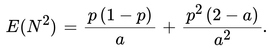
and the second moment
Hence the variance is (E(N^2) - [E(N)]^2), and the standard deviation (square root of the variance) simplifies to
Comprehensive Explanation
Overview of the Setup
Geometric Transmission Time The random variable T (the transmission time) follows a geometric distribution with parameter a. In practical terms, T represents the number of “time slots” needed to complete the transmission of a message. The key features of a geometric distribution with parameter a are:
Probability that T = n is a(1−a)^(n−1) for n = 1, 2, 3, ...
Expected value of T is 1/a.
This form of the geometric distribution counts the number of trials up to and including the first success. Here, each trial (time slot) succeeds in finishing the transmission with probability a.
Arrivals in Each Time Slot For every time slot, there is a Bernoulli trial with probability p of a new message arriving and (1−p) of no new message arriving. When T = n, we effectively have n Bernoulli(p) trials. Hence, given T = n, the number of arrivals N is Binomial(n, p).
Combining the Distributions Because T is itself random (geometric), we want the unconditional distribution of N. We use the law of total expectation and the law of total second moment to combine the Binomial(n, p) distribution (conditional on T = n) with the distribution of T.
Deriving the Expected Value E(N)
Conditional Expectation If T = n, then N ~ Binomial(n, p). So E(N | T = n) = n p.
Unconditional Expectation By the law of total expectation:
E(N) = sum_{n=1 to infinity} [ E(N | T = n ) * P(T = n) ].
In simpler terms: E(N) = sum_{n=1 to infinity} [ (n p) * a(1−a)^(n−1) ].
Factor out p:
E(N) = p * sum_{n=1 to infinity} [ n * a(1−a)^(n−1) ].
Next, recall the well-known series identity for 0 < (1−a) < 1:
sum_{n=1 to infinity} n r^(n−1) = 1 / (1−r)^2, where r = (1−a).
Hence,
sum_{n=1 to infinity} n (1−a)^(n−1) = 1 / a^2,
and multiplying by a gives a(1 / a^2) = 1/a. Therefore:
E(N) = p * (1/a) = p/a.
Deriving the Second Moment E(N^2)
Similarly, we use:
E(N^2) = sum_{n=1 to infinity} [ E(N^2 | T = n) * P(T = n) ].
Given T = n, N ~ Binomial(n, p), so
E(N^2 | T = n) = n p(1−p) + (n p)^2 = n p(1−p) + n^2 p^2.
Hence,
E(N^2) = sum_{n=1 to infinity} [ n p(1−p) + n^2 p^2 ] * a(1−a)^(n−1).
We can split this into two sums:
E(N^2) = p(1−p) * sum_{n=1 to infinity} [ n a(1−a)^(n−1) ] + p^2 * sum_{n=1 to infinity} [ n^2 a(1−a)^(n−1) ].
From above, sum_{n=1 to infinity} n a(1−a)^(n−1) = 1/a.
A known identity for the second sum is sum_{n=1 to infinity} n^2 r^(n−1) = (1+r)/(1−r)^3. Substituting r = (1−a) yields sum_{n=1 to infinity} n^2 a(1−a)^(n−1) = (2−a)/a^2.
Putting it all together:
E(N^2) = p(1−p) * (1/a) + p^2 * [(2−a)/a^2] = p(1−p)/a + p^2(2−a)/a^2.
Variance and Standard Deviation
The variance is Var(N) = E(N^2) − [E(N)]^2. We already have E(N) = p/a, so [E(N)]^2 = p^2/a^2. Therefore,
Var(N) = p(1−p)/a + p^2(2−a)/a^2 − p^2/a^2 = p(1−p)/a + p^2(1−a)/a^2 = [ p ( a(1−p) + p(1−a) ) ] / a^2.
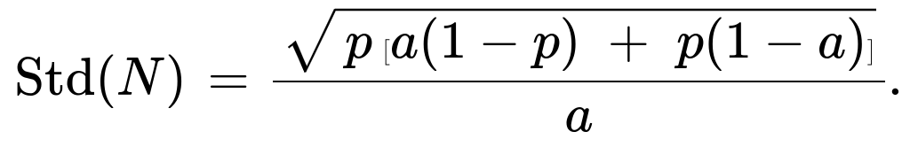
Taking the square root gives the standard deviation:
Std(N) = sqrt( Var(N) ) = ( 1/a ) * sqrt( p [ a(1−p) + p(1−a) ] ).
Hence, we arrive at the final concise results:
E(N) = p/a.
Std(N) = (1/a) * sqrt( p [ a(1−p) + p(1−a) ] ).
Potential Follow-Up Questions
1) Could there be a different parameterization of the geometric distribution and how would that affect E(N) and Std(N)?
Answer: Yes. Some texts define a geometric random variable as the number of failures before the first success, rather than the number of trials up to and including the first success. If we used that alternative definition, T would start at 0 rather than 1. In that case, the PMF becomes P(T = n) = a(1−a)^n for n = 0, 1, 2, ... and the expectation of T changes to (1−a)/a. That would shift the sums by one time slot, thus slightly modifying the sums for E(N) and E(N^2). However, because the original question explicitly uses the “starts at 1” version, we used the standard formula P(T = n) = a(1−a)^(n−1) with the first success counted in the total.
2) How do we interpret the result p/a in a real-world scenario?
Answer: In a real-world queue or communication system:
a is the success probability (per time slot) of completing the transmission, so on average it takes 1/a time slots to finish.
p is the probability a new message arrives in one slot.
Thus, over the average 1/a time slots, we expect p/a arrivals. Intuitively, if each time slot has p chance of an arrival, and you need on average 1/a time slots, then the total expected arrivals is just p × (1/a) = p/a.
3) What happens if p is very small or very large?
Answer:
If p → 0, then E(N) = p/a → 0. This makes sense: arrivals almost never happen, so in the time it takes to transmit, you almost surely get no new arrivals.
If p → 1, then E(N) = 1/a. You nearly always get a new message in each slot, so you are essentially counting all of those slots, giving you ~1/a new messages on average. The variance expression similarly adapts to that near-deterministic behavior when p is near 1.
4) What if a is very small or very close to 1?
Answer:
If a → 0, it means the transmission is highly unlikely to finish in a small number of time slots, so T is large on average (1/a becomes huge). Therefore, E(N) = p/a becomes very large. The standard deviation also grows significantly.
If a → 1, it means that you typically succeed on the first time slot, so T is often 1. Hence, E(N) = p/a → p, and N is either 0 or 1 (with high probability being 1). The standard deviation also shrinks accordingly.
5) Can we verify these results with a quick simulation in Python?
Answer: Yes. We can draw many samples of T from a geometric distribution, then for each T = n, draw N from Binomial(n, p). By averaging over many trials, we can empirically estimate E(N) and Std(N) and see that they match p/a and sqrt( ... ) / a.
import numpy as np

def geometric(a, size=1_000_000):
    # Returns number of trials up to/including the first success
    # with success probability a
    return np.random.geometric(p=a, size=size)

def simulate(a, p, num_samples=1_000_000):
    T_samples = geometric(a, num_samples)
    # For each T = n, sample from Binomial(n, p)
    N_samples = [np.random.binomial(n, p) for n in T_samples]
    mean_N = np.mean(N_samples)
    std_N = np.std(N_samples)
    return mean_N, std_N

# Example usage:
a_val = 0.3
p_val = 0.4
mean_est, std_est = simulate(a_val, p_val)
print("Estimated mean:", mean_est)
print("Estimated std :", std_est)

# Compare with theoretical:
theoretical_mean = p_val / a_val
theoretical_std  = (1.0/a_val) * np.sqrt( p_val*( a_val*(1-p_val) + p_val*(1-a_val) ) )
print("Theoretical mean:", theoretical_mean)
print("Theoretical std :", theoretical_std)
Such a quick simulation confirms the correctness of the derived formulas empirically.
6) Why do we split E(N^2) into two parts when computing the variance?
Answer: When T = n, we know N is Binomial(n, p), and so
E(N) = n p
E(N^2) = n p(1−p) + (n p)^2
To combine these with the geometric distribution for T, we sum over n = 1..∞ weighted by the geometric pmf. It is typically easier to sum over each term separately (one for n p(1−p), one for n^2 p^2) and use known series expansions for Σ n r^(n−1) and Σ n^2 r^(n−1).
7) Could we use moment generating functions (MGFs) to solve this instead?
Answer: Yes, one can use moment generating functions:
The MGF of N given T=n (Binomial(n, p)) is (1−p + p e^t)^n.
Then average this MGF over the distribution of T (geometric with parameter a).
Differentiate the resulting MGF to get the first and second moments.
Though more involved, it leads to the same expressions for E(N) and E(N^2), confirming the result.
These details cover both the direct summation approach and some alternative strategies (MGF, simulations), along with edge cases and real-world intuition for the expressions p/a and the corresponding standard deviation.
Below are additional follow-up questions
What if the arrival probability p changes over time rather than staying constant?
When we derived E(N) = p/a, we implicitly assumed that p is a fixed probability for each time slot. In reality, though, the arrival probability might depend on the slot index. For instance, early time slots could have a lower p, and later time slots might have a higher p, or vice versa. If p depends on n (the slot index), then:
Conditional on T = n, N would be the sum of n Bernoulli random variables, but these Bernoulli parameters would differ across time slots (say p1, p2, …, pn instead of a constant p).
The conditional expectation E(N | T = n) then becomes the sum of those probabilities: p1 + p2 + … + pn.
The unconditional E(N) is obtained by summing over the geometric distribution for T = n. That is:
E(N) = sum_{n=1 to infinity} [ (p1 + p2 + … + pn) * a(1−a)^(n−1) ].
This would require specifying exactly how p changes with n. If p(n) is a decreasing function or increasing function, the resulting series could be more complicated. One would need to carefully evaluate that sum to find an explicit closed-form solution—if it exists. If it does not simplify easily, one might rely on numerical approximation or simulation methods.
A potential pitfall is assuming we can still just multiply an “average p” by the mean T. That only works if T is independent from the distribution that determines p(n). But if T’s magnitude somehow correlates with the arrival probabilities, you need a more careful approach (for instance, if p(n) changes in a way that’s systematically related to how many slots are likely to occur).
What if more than one new message can arrive in a single time slot?
In the problem setup, exactly one new message arrives with probability p, and zero arrives with probability 1−p, in each slot. However, in many real systems, there can be multiple arrivals in a single time slot. If we replace the Bernoulli arrival process with a more general distribution (e.g., a Poisson(lambda) distribution of arrivals per slot), then:
Conditional on T = n, N would be the sum of n i.i.d. Poisson(lambda) random variables, which is itself Poisson(n * lambda).
E(N | T = n) = n * lambda.
Then E(N) = sum_{n=1 to infinity} [ (n * lambda) * a(1−a)^(n−1) ] = lambda * (1/a) = lambda / a.
The second moment and variance derivations would also mirror the procedure we used, but substituting in the known second moment for Poisson. Specifically, E(N^2 | T = n) = nlambda + (nlambda)^2 for Poisson(n lambda). Summing that series with the geometric distribution for T would yield the unconditional E(N^2).
A subtlety is that if the number of arrivals per slot can be unbounded, the variance can grow differently than in the Bernoulli case, influencing system performance in queueing or throughput scenarios. Thus the next pitfall is blindly using the Bernoulli-based formula for E(N^2) or Var(N). One must recompute these moments for the actual arrival distribution used.
What if the system experiences correlation between arrivals in different slots?
The derivation for E(N) and E(N^2) assumes each slot is independent, with a new message arriving with probability p. If, instead, arrivals across time slots are correlated (for example, arrivals might come in bursts followed by periods of no arrivals), then N is no longer a sum of independent identically distributed Bernoulli random variables. The binomial model would fail to capture the correlation structure.
A pitfall here is to assume the binomial distribution remains valid if arrivals across slots are correlated. That can significantly alter the distribution of N given T = n.
If correlation is positive, we might see larger bursts, and the variance of N can be higher than the binomial-based calculations predict.
If correlation is negative (for instance, if arrivals in one slot reduce the chance of arrivals in subsequent slots), the variance could be smaller.
A thorough approach would be to model the joint distribution of arrivals across all time slots or use more advanced queueing theory frameworks (like Markov modulated processes) that capture correlation.
Could random variables T and the arrival process be dependent?
In the standard problem, T is purely geometric with parameter a, and the arrival events for new messages occur independently of T’s progression. In some real-world processes, the chance to finish transmission (probability a) might depend on how many arrivals occur or how congested the system is. For instance, if more new messages arrive, it might slow down the channel or cause collisions, altering the probability that the transmission completes in a slot.
This introduces the possibility that T and N are not independent: the value of T might be larger precisely when more arrivals happen.
If T has some dependency on whether new arrivals occur, the geometric assumption for T = n might break down, or we would have a different parameter a(n) that changes over time or depends on arrivals.
The law of total expectation approach still works in principle, but E(N | T = n) might not simply be n p. One would have to carefully define that conditional distribution, or model T’s distribution in a way that accounts for these feedback effects.
The pitfall is ignoring these dependencies and treating T and N as though they are independent processes when they’re not, which leads to incorrect moment calculations.
How do these results extend to continuous-time settings?
The problem is phrased in discrete time slots (each slot we either succeed in transmitting with probability a, or not). A continuous-time analog might have an exponential distribution for the “inter-transmission time” (exploiting the memoryless property), and arrivals might follow a Poisson process with rate lambda:
Then T ~ Exponential(mu), for some rate mu. The mean T would be 1/mu.
Number of arrivals in time T is Poisson(lambda T). Conditioned on T = t, the expected arrivals is lambda t.
Unconditionally, E(N) = lambda * E(T) = lambda/mu.
Though the numerical result might look similar to the discrete-time ratio p/a, the derivations proceed via integration rather than summation. The memoryless property of the exponential distribution plays a similar role to that of the geometric distribution in discrete time.
A subtlety arises if the system is not truly memoryless. For instance, if the distribution of T is not exponential, or arrivals are not Poisson, the computations require more advanced formulas. The pitfall is to apply exponential or Poisson assumptions blindly without verifying they match the actual process behavior.
What practical implementation pitfalls might arise in coding or simulation?
When simulating T from a geometric distribution:
One might mistakenly use a naive approach to generate T that leads to performance issues for small a, because T can become very large. Repeatedly sampling trial outcomes can be inefficient. A more efficient approach is to use
np.random.geometricor an equivalent built-in geometric sampler.For large sample sizes, floating-point arithmetic can introduce minor numerical instability, especially when summing a(1−a)^(n−1) for large n.
In computing second moments or variances empirically, a large enough sample is critical, because tail events (especially for very small a) can be rare but heavily influential.
A pitfall is to do a “quick test” with too few samples, thus severely underestimating or overestimating the variance. Another issue is misidentifying the parameterization of the geometric distribution in code. Some libraries define geometric as “the number of failures before the first success,” while others define it as “the number of trials up to the first success.”
Is it possible for N to equal zero even if T is large?
Yes, it is entirely possible. For each time slot, a new message arrives with probability p, but with probability (1−p) no new message arrives. Even if T is large, you could get zero arrivals if the Bernoulli random draws fail each time. The probability that N = 0 given T = n is (1−p)^n. Summing over the distribution of T, the overall probability of zero arrivals is:
sum_{n=1 to infinity} [ (1−p)^n * a(1−a)^(n−1) ].
This sum is not zero unless p = 1. In real applications, that means you can have an arbitrarily long transmission period during which no new messages arrive—though it might be unlikely for large n if p is moderate or large. The pitfall for a system designer is failing to account for the rare (but nonzero probability) event that no arrivals appear for many slots, which might affect how the system times out or restarts transmissions.