ML Interview Q Series: Analyzing EV Lifetime Differences: Probability Calculation with Gaussian Distributions.

Browse all the Probability Interview Questions here.
8. Say that the lifetime of electric vehicles is modeled using a Gaussian distribution. Each type of electric vehicle has an expected lifetime and a lifetime variance. Say you choose two different types of electric vehicles at random. What is the probability that the two lifetimes will be within n time units?


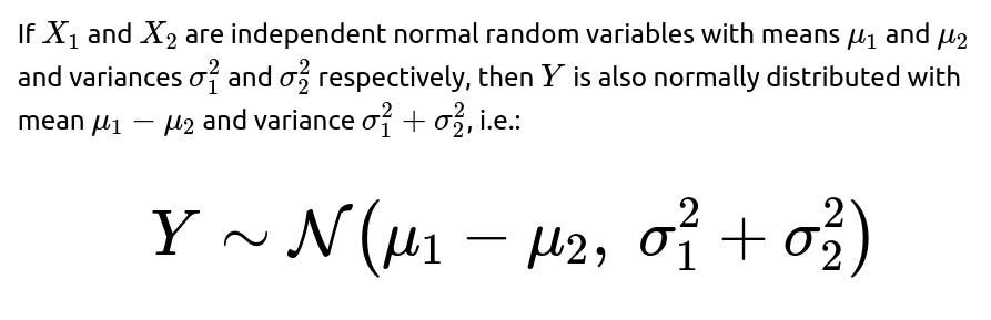


This expression is the probability that the difference of two normally distributed lifetimes falls within the interval [−n,n].

import math
import numpy as np
from scipy.stats import norm
def probability_within_n_units(mu1, sigma1, mu2, sigma2, n):
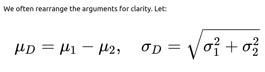
mu_diff = mu1 - mu2
sigma_diff = math.sqrt(sigma1**2 + sigma2**2)
# Lower bound and upper bound in terms of the standard normal
lower_z = (-n - mu_diff) / sigma_diff
upper_z = (n - mu_diff) / sigma_diff
return norm.cdf(upper_z) - norm.cdf(lower_z)
# Example usage:
mu_1 = 100.0 # Example mean for vehicle type 1
sigma_1 = 10.0 # Example std dev for vehicle type 1
mu_2 = 105.0 # Example mean for vehicle type 2
sigma_2 = 12.0 # Example std dev for vehicle type 2
n_val = 5.0 # We want the probability that the two lifetimes differ by <= 5.0
prob = probability_within_n_units(mu_1, sigma_1, mu_2, sigma_2, n_val)
print("Probability that the two lifetimes are within 5.0 units: ", prob)
This completes the direct solution. However, in a real FANG-type interview, there could be numerous follow-up questions that delve into assumptions, edge cases, potential generalizations, and real-world scenarios. Below are some typical follow-up questions an interviewer might ask, along with detailed explanations and potential pitfalls.
What if the two lifetimes are correlated?


What if there are outliers in the data or the distribution is not strictly Gaussian?
While we assumed a Gaussian distribution, real-world data can be heavy-tailed (i.e., contain outliers or extreme values that occur more frequently than the normal distribution predicts). Electric vehicle lifetimes could be subject to factors such as manufacturing defects or usage anomalies that create a longer tail.
One possible approach is to test whether the lifetime data fits a Gaussian well (for instance, using Q-Q plots or statistical tests). If the fit is poor, you might consider other distributions like lognormal or gamma distributions. If you persist in using the normal distribution despite heavy tail behavior, the probability estimate might be overly optimistic or pessimistic about differences in lifetimes.
A common pitfall is ignoring how outliers can affect the estimated mean and variance. If a handful of extreme data points significantly inflates the sample variance, the probability of being within n might become underestimated, or vice versa.


How would we address the question if the lifetimes were lognormally distributed?

How to handle scenarios where data is incomplete or censored?
In some real-world situations, you might not fully observe the entire lifetime of every vehicle. Certain vehicles might still be operating, leading to right-censored data, or you might not know the exact start time for usage, leading to left-censored data. If the data is censored, you need specialized statistical methods (e.g., survival analysis techniques such as Kaplan-Meier estimates or parametric survival modeling) to properly estimate the distribution parameters.
A typical pitfall is ignoring censorship and treating partially observed lifetimes as if they were complete, which biases the means and variances. Correctly accounting for censorship is especially important if only a fraction of the vehicles have reached their "end-of-life" events.
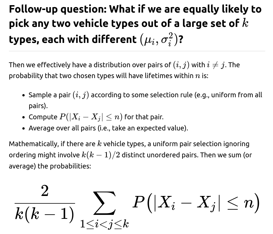
Could we extend this to more than two vehicle types?
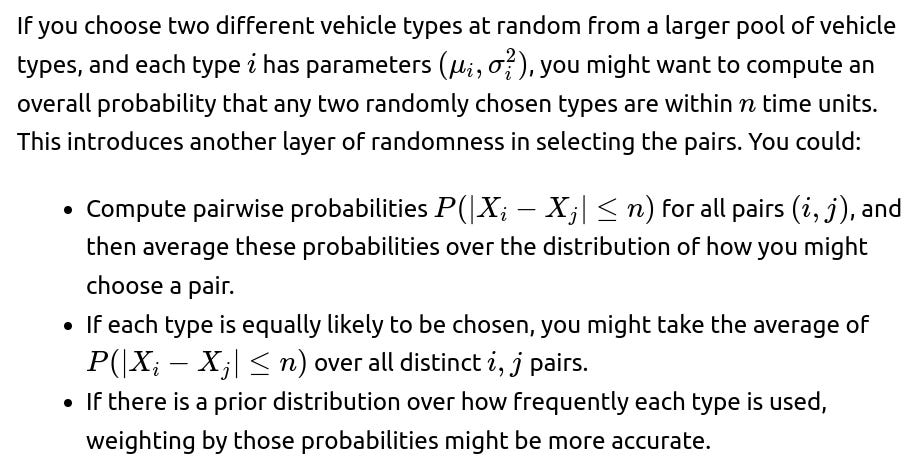
Pitfalls include incorrectly weighting or ignoring how often a type is actually chosen in practice. Also, as you aggregate over many types, differences in data quality or differences in usage conditions can complicate parameter estimates.
Implementation details and practical considerations
In actual implementation, especially if you have large amounts of data, you will likely:
Collect lifetime data for each vehicle type.
Perform basic data cleaning (removing impossible values, dealing with missing or censored data).
Estimate mean and variance carefully, possibly using robust statistical methods if outliers are present.
Plug the estimates into the derived formula for the difference of two Gaussians, or use more general simulation/numerical methods if the distribution is not normal or if correlation is present.

How would you validate the result in a real-world scenario?
Interviewers might probe how you would confirm that the computed probability is not purely theoretical but also valid in a production setting:
Compare the computed probability to actual differences observed in a hold-out or test dataset.
Use a bootstrapping approach: sample from your empirical distribution many times, compute the fraction of pairs whose difference is within n, and see how well it matches the theoretical formula.
Track actual usage and retirements of vehicles over time. If data consistently disagrees with your model’s predictions, investigate whether the distributional assumptions or parameter estimates are incorrect or have shifted over time (e.g., changes in manufacturing processes or usage patterns).
Potential pitfalls and summary of key ideas
Independence vs. correlation. If your vehicles share manufacturing lines, usage conditions, or other correlated factors, ignoring correlation can give a wrong probability.
Distribution assumptions. Gaussian might be a convenient approximation, but it could be inaccurate if the real data is heavily skewed or has long tails.

Real-world complexities. Censored data, changing usage patterns, or not having enough historical data can introduce errors.
Validation. Always verify theoretical results using real or simulated data to ensure the model is producing correct probability estimates for the difference in lifetimes.
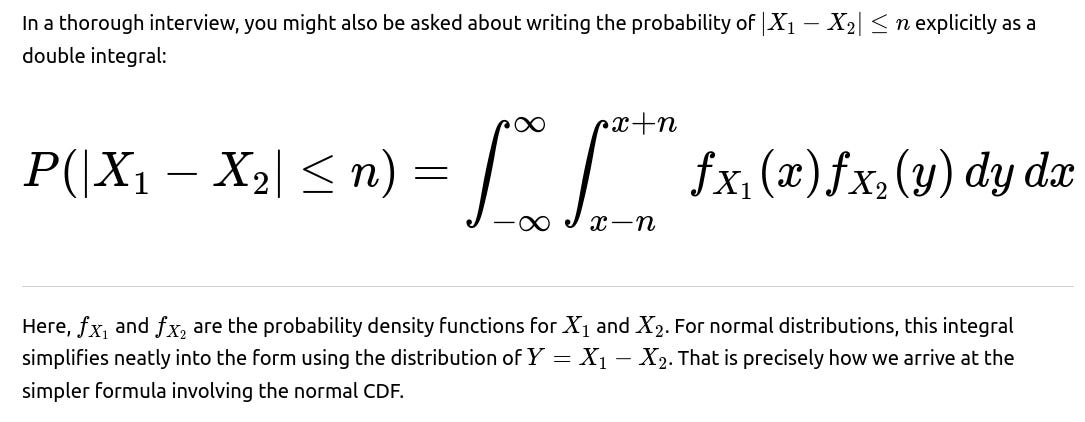
What if an interviewer wants the explicit integral representation?

Additional subtle real-world questions an interviewer might ask

These sorts of considerations demonstrate both the mathematical foundation of the probability computation and the nuanced real-world constraints that might come into play in a FANG interview.
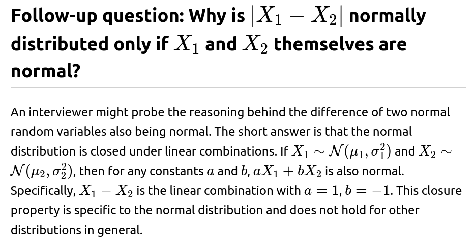
Follow-up question: What if the two lifetimes are correlated?
If the lifetimes are correlated with correlation coefficient ρ, then:

Follow-up question: What if the distribution of lifetimes is not actually Gaussian?
Many real-world processes do not follow a strict Gaussian distribution. Lifetimes, in particular, can be skewed. If the underlying distribution is unknown or suspected to be non-Gaussian, you can:

A main pitfall is forcing a normal distribution on a dataset that is significantly skewed or has heavy tails. This can drastically underestimate or overestimate probabilities in the tails, leading to poor real-world predictions of differences in lifetimes.
Follow-up question: How do we handle limited sample sizes for estimating means and variances?
With limited data, the sample estimates of mean and variance might be very uncertain. Some strategies:

Follow-up question: In practice, how do we interpret this probability?
If an interviewer wants clarity on practical interpretation, you might say: “Given the distribution of lifetimes for these two types of vehicles, we have a certain confidence region that these lifetimes will differ by no more than n. This is useful if, for example, we want to ensure that two deployed models of vehicles have ‘comparable lifetimes’ for marketing or warranty overlap. It gives a single numeric measure: the fraction of all possible pairs of vehicles (one from each type) that would differ in lifetime by ≤n.”
Pitfall is to interpret it as a guarantee for every single vehicle. Probabilities are about overall distributions. In reality, some vehicles might differ by more than n time units, but the fraction of such occurrences is what the computed probability seeks to quantify.
Follow-up question: Could we use empirical simulation to verify the formula?
Yes. If you have large enough samples from each distribution:

If they match closely, it suggests your assumptions are holding. If not, investigate whether the distribution is not normal, if there is correlation, or if your estimates of mean and variance are off.

Follow-up question: What if the question asked for the probability that the sum of the lifetimes is within some bound?

So the sum is straightforward if they are independent normals, but conceptually it is different from the difference we examined.
Potential confusion arises if an interviewer flips the scenario from difference to sum. The details remain the same in the sense that normal distributions are closed under addition, but the question addresses a different event. In warranty or cost analysis, sometimes the sum matters (e.g., total usage across two subsystems). In comparing two lifetime durations for equivalency, the difference typically matters.

Follow-up question: Could you show a quick numerical demonstration?

import numpy as np
from scipy.stats import norm

np.random.seed(42)

mu1, sigma1 = 100.0, 10.0
mu2, sigma2 = 105.0, 12.0
n_val = 5.0
num_samples = 10_000_000  # Large enough to reduce Monte Carlo error

# Generate samples
samples_x1 = np.random.normal(mu1, sigma1, num_samples)
samples_x2 = np.random.normal(mu2, sigma2, num_samples)

# Empirical estimate
diffs = np.abs(samples_x1 - samples_x2)
empirical_prob = np.mean(diffs <= n_val)

# Theoretical estimate
mu_diff = mu1 - mu2
sigma_diff = np.sqrt(sigma1**2 + sigma2**2)
cdf_lower = norm.cdf((-n_val - mu_diff)/sigma_diff)
cdf_upper = norm.cdf((n_val - mu_diff)/sigma_diff)
theoretical_prob = cdf_upper - cdf_lower

print("Empirical Probability:   ", empirical_prob)
print("Theoretical Probability: ", theoretical_prob)
In a well-behaved scenario with many samples and correct parameterization,
empirical_probandtheoretical_probwill be close, providing reassurance that the analytical result and simulation match.Follow-up question: How do we interpret potential discrepancies between the empirical estimate and the theoretical probability?
If in the simulation you observe a large discrepancy, typical reasons include:

In an interview, demonstrating an awareness of these factors indicates a practical understanding of how to validate models in real-world conditions.

The factor of 2 accounts for either ordering if the question truly picks “two different types” in a way that does not distinguish who is first or second; specifics can vary. This scenario can become more complicated if each type is chosen with a different probability.

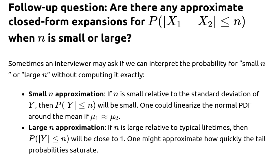
But typically, the direct normal CDF approach is straightforward enough that approximate expansions are less commonly used in code—though discussing them can demonstrate your understanding of asymptotic behavior.
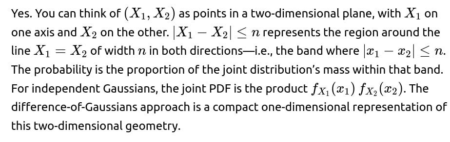
Follow-up question: Is there a geometric or intuitive interpretation?
Follow-up question: Are there any real-world engineering implications?
One might want to see if two vehicles, each from different manufacturers, have sufficiently comparable lifetimes for combined fleets or extended warranties. Or perhaps a fleet manager wants to interchange certain parts across brands only if they are likely to wear out at about the same time. The question “are these lifetimes within n of each other?” is fundamentally about operational planning, inventory management, or marketing claims about parity in longevity.
The probability helps quantify the risk of large discrepancies. For instance, if the question is: “With what probability will two random vehicles have lifetimes within 6 months of each other?” a company might use that to decide if it can unify warranty policies. If that probability is very high, it might be feasible to treat them uniformly. If not, they may need separate policies or disclaimers.
Follow-up question: Summary of the final formula and logic?
The final formula, under the assumptions of independence and normality, is:

We interpret it as the area under the difference-of-normals distribution from −n to n. This approach is standard and widely used because of the linear properties of the normal distribution. All complexities or “twists” in interview questions revolve around validating normality, independence, parameter estimation, and generalizing to correlated or non-normal distributions.


Below are additional follow-up questions
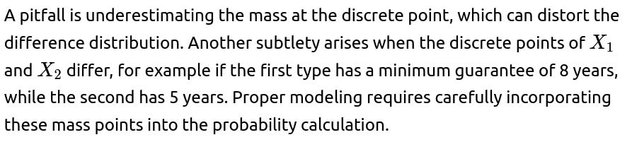
What if the lifetimes are partially discrete, such as when vehicles have a minimum guaranteed lifetime?
One could encounter a scenario where the manufacturer guarantees a minimum lifetime (for instance, a warranty period). Below that time, it is effectively impossible for a vehicle to fail, which introduces a mass point at that minimum threshold. Beyond the minimum threshold, the vehicle’s lifetime might follow a continuous distribution. This type of partial discreteness can occur in practical situations, such as contractual guarantees or design constraints that eliminate early failures.

If both random variables have a mass at specific points, you need to account for that probability spike separately. For any continuous parts, you can convolve or use difference-of-variables logic. But for any mass points, you sum the probability that each variable lands in a discrete mass, then see if the difference in that scenario is within n. Practically, you may need to:
Gather enough data to estimate:
The probability mass at the guaranteed minimum lifetime.
The conditional distribution above that minimum.
The correlation or dependence structure, if any, between the discrete occurrences.

How could we use quantiles or rank-based approaches to assess if the difference is within n?
Sometimes, especially for robust statistics, you might want to avoid relying purely on parametric assumptions about normality. Instead, you could use quantile-based approaches. You might do this by:

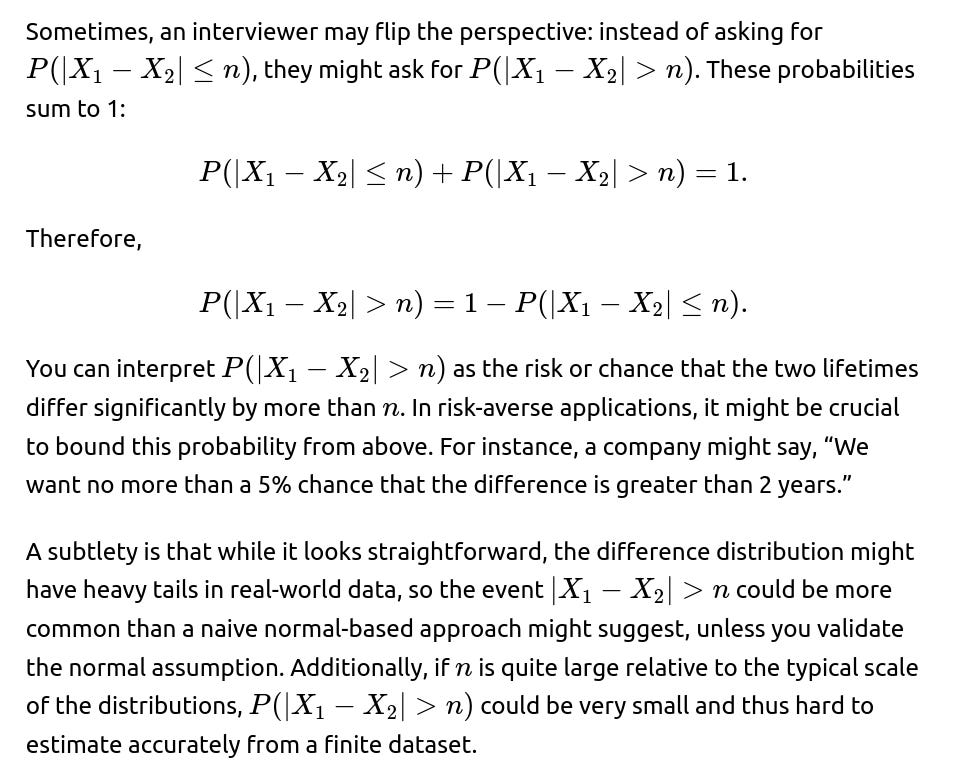
How do we reinterpret the probability if we are interested in the complement event, i.e., that the difference exceeds n?

How would a Bayesian approach treat the distribution of the difference?


From that predictive distribution, you can compute P(∣Y∣≤n). This can be done via Monte Carlo methods (sample parameters from their posteriors, then sample from the difference distribution). The advantage is that parameter uncertainty is properly accounted for. A pitfall is that Bayesian modeling can become computationally demanding, and one must choose priors carefully to avoid spurious or overly strong beliefs about the lifetimes. Also, if the dataset is large, one might default to frequentist estimates; but the Bayesian route can be especially illuminating when sample sizes for certain vehicle types are limited.
How do physical constraints like vehicles not having negative lifetimes or extremely large lifetimes impact modeling?
In reality, a vehicle cannot have a negative lifetime, and there may be practical upper bounds (though that upper bound might be quite large). Gaussian distributions are unbounded. While negative values might have negligible probability if μ is large relative to σ, the normal distribution is not strictly appropriate for random variables with limited support.
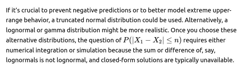
A pitfall arises if you blindly apply the normal formula for differences near domain boundaries (like near zero). You might see physically impossible results or large errors in tail probabilities. In some engineering contexts, even a small estimated probability of negative lifetime is a big red flag that the model is incomplete or incorrectly specified.
How do time-varying hazard rates in reliability analysis affect the probability that lifetimes differ by at most n?
In advanced reliability engineering, lifetime is often modeled via hazard functions that can change over time. For instance, early in the vehicle’s life, the hazard of failure might be low (“infant mortality” issues aside), then it might rise after the battery or motor degrades over several years, and eventually flatten. If each vehicle’s lifetime distribution is derived from a non-constant hazard function, it may not neatly fit the normal distribution.

A subtlety is that for certain hazard functions, the distribution might be heavily skewed. Another subtlety is how operating conditions might shift hazard rates in correlated ways. Relying on a naive normal approach could be very misleading. So the main pitfall is ignoring the time-varying nature and simply plugging in a normal approximation derived from partial data.
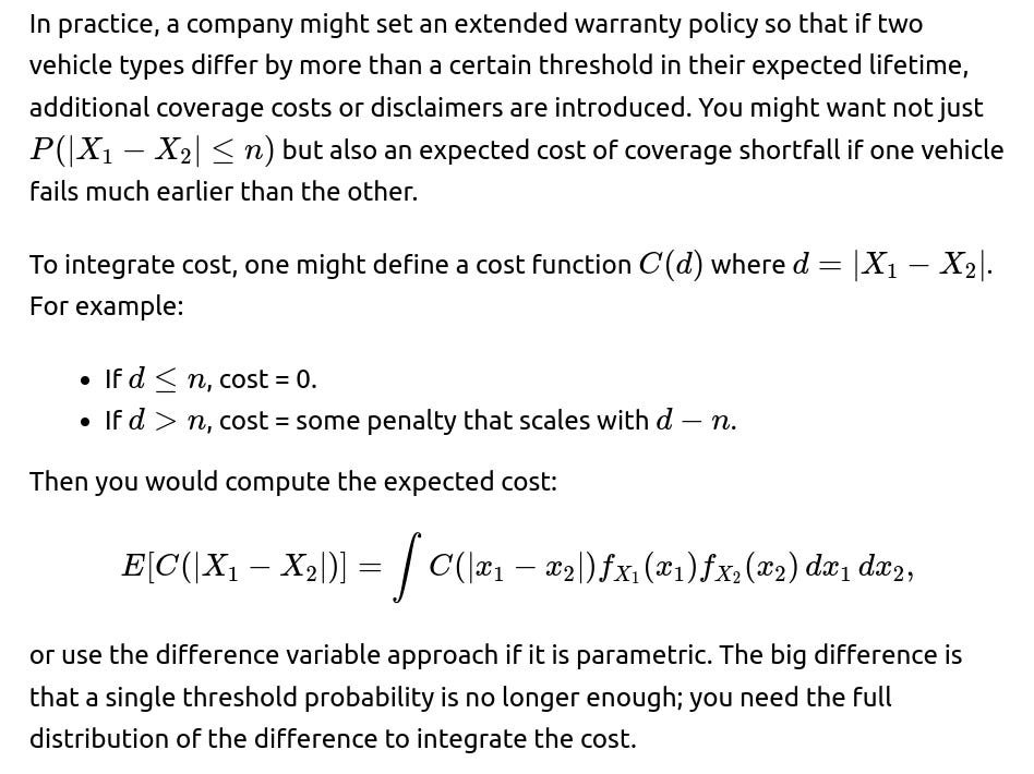
How do we handle a scenario where the difference in lifetimes is used in a cost model for extended warranties?

Could large sample sizes allow a normal approximation even if individual lifetimes are not normal?
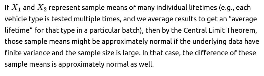
A subtlety: This is different from saying each individual vehicle’s lifetime distribution is normal. Instead, you’re using a normal approximation for the distribution of the sample mean. This is especially common in aggregated or manufacturing test data. The pitfall is that if the sample sizes are not large enough or if the underlying distribution is extremely skewed or heavy-tailed, the normal approximation might still be poor, especially in the tails.
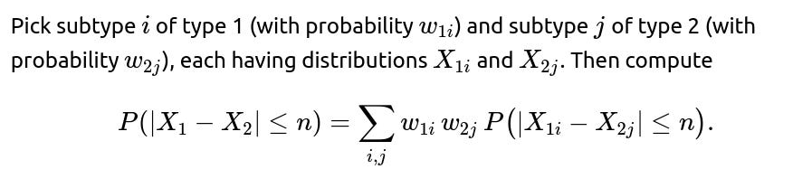
How does one handle a hierarchical scenario where each vehicle type has subtypes with different distributions?
In some real-world contexts, each broad “type” of electric vehicle might be subdivided into multiple sub-models or trim levels, each with a slightly different battery or motor design. One might consider a hierarchical (multilevel) model:
You estimate parameters at the subtype level and have hyper-parameters for the overall type. The difference in lifetimes between two broad types then marginalizes over the distribution of subtypes in each. Formally, you could do:

A pitfall is ignoring the within-type variability. If you treat each broad type as a single distribution, you might over-smooth differences, missing the fact that certain subtypes within a type might have drastically shorter or longer lifespans. Another pitfall is incorrectly aggregating subtypes that have wide variance. For a thorough approach, confirm that subtypes are truly exchangeable enough to be grouped hierarchically.
How do mixture distributions for the lifetimes affect the difference?
You might discover that each vehicle type’s lifetime is best modeled by a mixture of different normal components. For instance, 70% of vehicles might fail around 8–9 years, while 30% might be extremely robust and last 12+ years. Each type thus has a mixture distribution. The difference of two mixture distributions becomes even more complicated. If:

How do we incorporate evolving distribution parameters if manufacturing processes improve over time?

Pitfalls: If you treat the entire lifetime data as a single stationary dataset, you might ignore improvements or degrade data from older versions that do not reflect the current product. Also, a mismatch in production times for the two vehicle types can strongly affect how similar their lifetimes are. Failing to account for that can systematically bias your probability estimate.

A pitfall is that if the distribution changes (due to new manufacturing processes or usage patterns), a naive streaming approach that lumps old and new data might produce incorrect estimates. You may need to detect concept drift and “forget” old data or weight it less. This complexity might be tested in an interview to see if you appreciate that streaming data can break stationarity assumptions.
How does the probability change if we shift from comparing mean lifetimes to comparing median lifetimes?

How do we handle a scenario where we care about the ratio of the two lifetimes rather than the difference?

For a ratio of two independent lognormal variables, you might again get a lognormal ratio. But for normal variables, the ratio is related to the Cauchy distribution if the means are zero, though that’s typically not the scenario for lifetimes. You might:
Transform each to a log scale if that better suits the data.
Use simulation to estimate the ratio probability.
In some specialized cases, use known ratio-of-normals distributions if you can handle restricted parameter spaces.

What if we suspect partial correlation but cannot reliably estimate ρ?

A pitfall is ignoring correlation altogether. Another pitfall is plugging in a guessed ρ that’s not empirically justified. If the interview asks about how to handle uncertain correlation, an appropriate response might be to gather more data or identify an external data source that clarifies the dependence structure. Or, if pressed for time, at least produce an interval of probable outcomes under different correlation scenarios, so decisions can be made robustly.

A subtlety is that if your sample size is small or your distributions heavily skewed, the confidence interval might be wide. Another subtlety is that if you fail to incorporate correlation or other real-world complexities, your interval might be misleadingly narrow. This question tests whether you understand that the final probability is itself an estimate with uncertainty, not just a single number from a formula.
How might an “infant mortality” phenomenon for electric vehicles complicate the difference distribution?

A subtle pitfall is ignoring the sub-population that fails early. That sub-population might cause a relatively large absolute difference if one type is more prone to early failure. Another issue is correlation if the usage environment that triggers early failures affects both types similarly. The interviewer might ask whether you have a plan to gather enough data on that early-failure sub-population to model it accurately.
How could we handle a max or min scenario instead of a difference?

A subtlety is that if you misinterpret “difference” for “max” or “min,” you get the wrong probability. Another subtlety is if they are correlated. Then you can’t just multiply probabilities. This question might appear if an interviewer wants to see if you can pivot from difference-based questions to other functionals of random variables.
How to deal with significant differences in sample sizes for the two vehicle types?

If the interviewer wants to see a direct synergy between theory and simulation in real time, how do we proceed?

Generate synthetic data for each vehicle type.
Estimate the fraction of pairs whose difference is within n.
Compare it to an analytical formula (if one exists).
Check how that fraction changes if you vary n.
This synergy demonstrates practical modeling skills. A subtlety is that for distributions without a closed form, simulation might be the main tool. Another subtlety is ensuring you sample from the correct distribution. If you mismatch parameters or correlation structure, your results might be invalid. The interviewer is often checking if you can connect the theoretical approach to an applied, experimental approach that validates or refines your understanding.